Clear Graphical and Mathematical Explanation of Euler Angles – Part 1

In this rigid body dynamics, GNC (guidance, navigation, and control), and physics tutorial, we provide a clear explanation of Euler angles. In this tutorial, we focus on the so-called Z-X’-Z” Euler angles, and in the second part of this tutorial, we will focus on the Yaw-Pitch-Roll Euler angles. The YouTube tutorial accompanying this post is given below.

Mechanism of Euler Angles

Before we start with explanations, we need to explain the main motivation for creating this tutorial. There are a large number of books on robotics, dynamics, and aerospace topics that cover Euler angles. However, in these books, Euler angles are not properly and clearly graphically explained. Equations are immediately introduced without providing students with the necessary graphical and intuitive understanding of Euler angles. Due to this, in this tutorial, we dedicate special attention to the graphical understanding of Euler angles.

Euler angles are used in many applications. Generally speaking, we use Euler angles to represent the orientation of a rigid body in space. In aerospace applications, orientation is also called attitude. What is the orientation of a rigid body? The orientation of the rigid body is a sequence of rotations with respect to some fixed or translating frame that is used to uniquely define the current rotational state (orientation) of the body. For example, let us assume that we have a body that can rotate with respect to its center of mass. Then, let us arbitrarily rotate this body. Its orientation is a set of mathematical parameters that uniquely describe the current state of rotation of the body with respect to the fixed or inertial frame.

There are several approaches for selecting parameters that describe the orientation of a rigid body. One of the approaches is to use the Euler angles. Euler angles are three angles that are used to sequentially rotate three axes of a rigid body. By using Euler angles we can mathematically describe any rotational state or orientation of a rigid body. That is, Euler angles are used to mathematically represent, or better to say, define the orientation of a rigid body with respect to some coordinate system that is used as the reference.

In addition to three Euler angles, we need additional three parameters to completely define the position and orientation of a rigid body in space. The position of a rigid body in the space is described by three parameters. They are , , and coordinates of the center of the mass of the body.

In the sequel, we thoroughly explain the concept of Euler angles. However, we suggest that you first watch the following video tutorial that graphically explains three Euler angles and three sequential rotations produced by Euler angles.

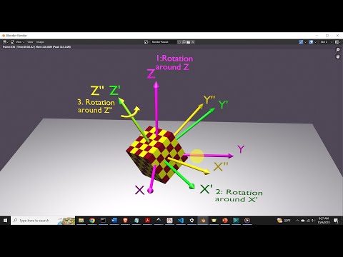
Next, we thoroughly explain the Euler angles and induced rotations. The graph given below explains the Euler angle convention.

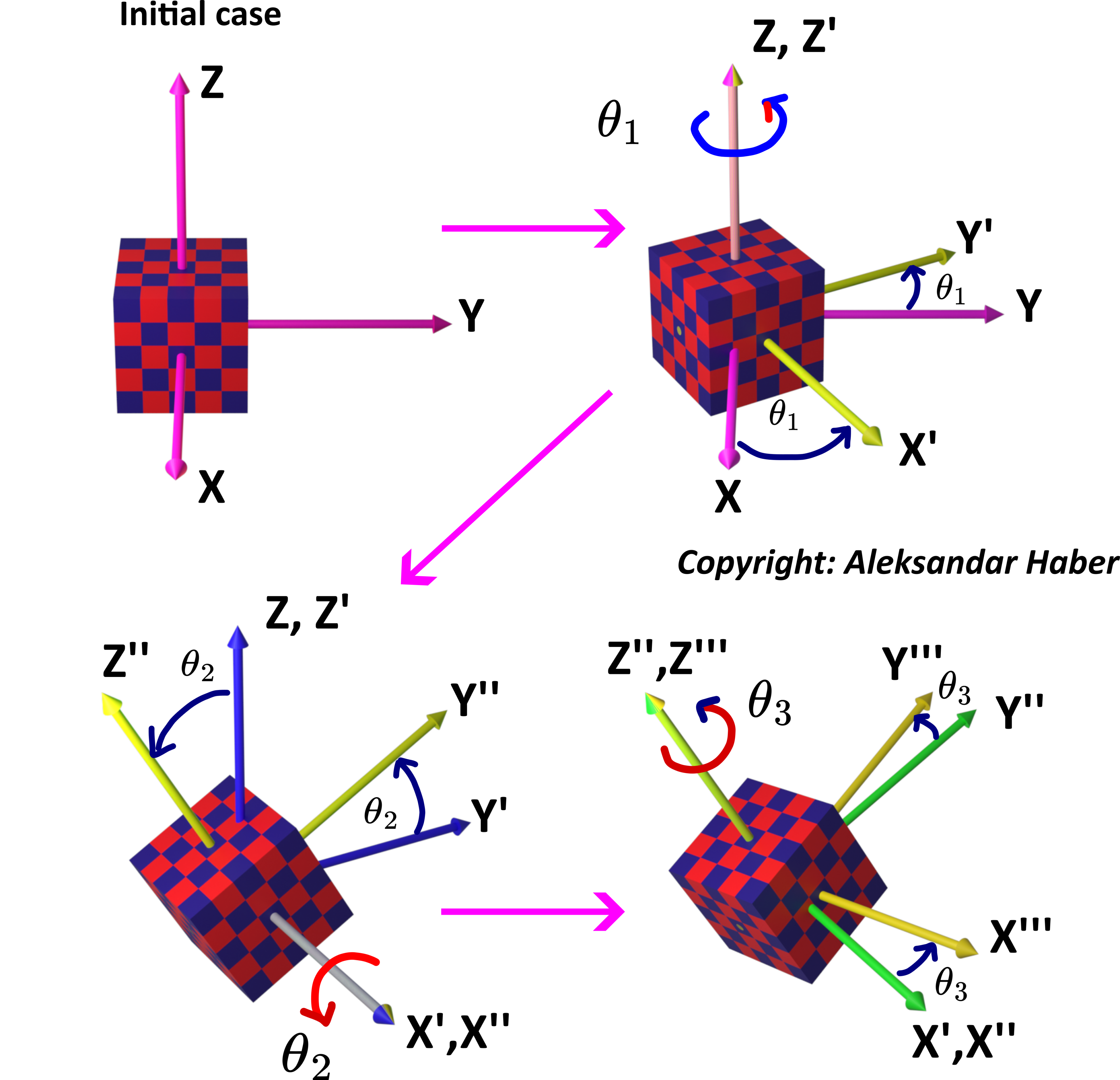
This figure shows a 3D cube that is sequentially rotated 3 times. The initial coordinate system is centered at the center of the mass of the cube. The Euler angle rotations are described as follows:

1. In the first rotation, we rotate the cube around the axis. The rotation angle is . This rotation defines a new coordinate system .
2. Then, we rotate the cube around the axis. The angle or rotation is . This rotation defines a new coordinate system .
3. Finally, we rotate the cube around axis. The angle or rotation is . This rotation defines the final coordinate system . We performed three sequential rotations.

The angles and are called the Z,X’,Z” Euler angles. They are also called Euler angles. The notation or denotes the sequential axes of rotation. There are also other ways for defining the Euler angles by using other axes of rotation. However, more about this in our future tutorials.

Let us introduce the following notation for the coordinate systems in order to simplify the mathematical notation in the sequel:

• The coordinate system is denoted by .
• The coordinate system is denoted by .
• The coordinate system is denoted by .
• The coordinate system is denoted by .

The Euler angles with the new notation for coordinate systems are shown in the figure below.

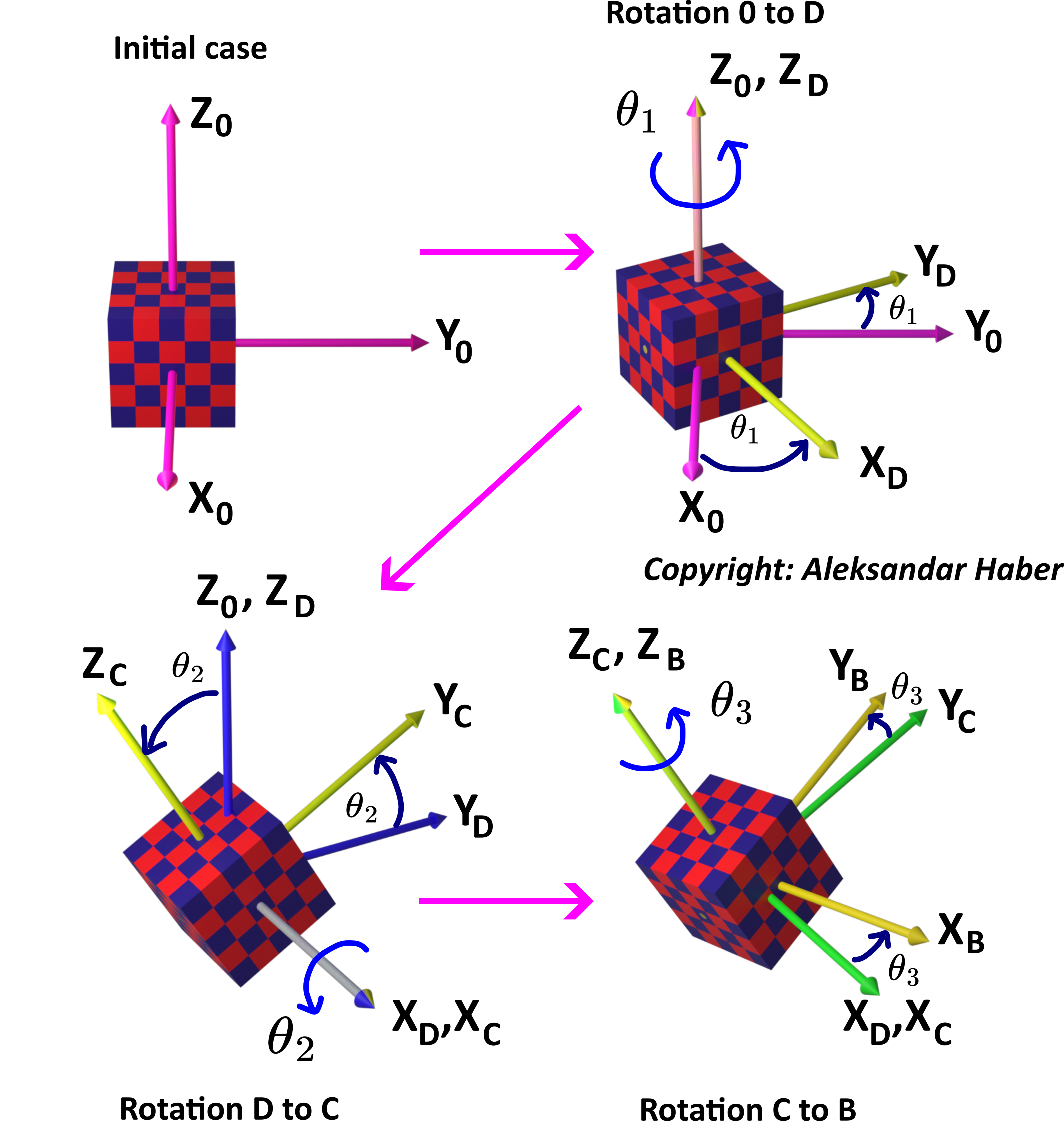
Here, we should mention the following. The coordinate system is the so-called body coordinate system and its direction is always in the direction of the principal axes of the body (axes of symmetry in our case). This coordinate system is rigidly attached to the body. In the initial configuration, this coordinate system coincides with the coordinate system 0. Then, after the first rotation, this coordinate system coincides with . Then, after the second rotation, this coordinate system coincides with .

Next, let us introduce the following notation. Let be a vector. Then, the notation is the notation for the vector expressed in the coordinate system with the following projections in the coordinate system :

(1)  

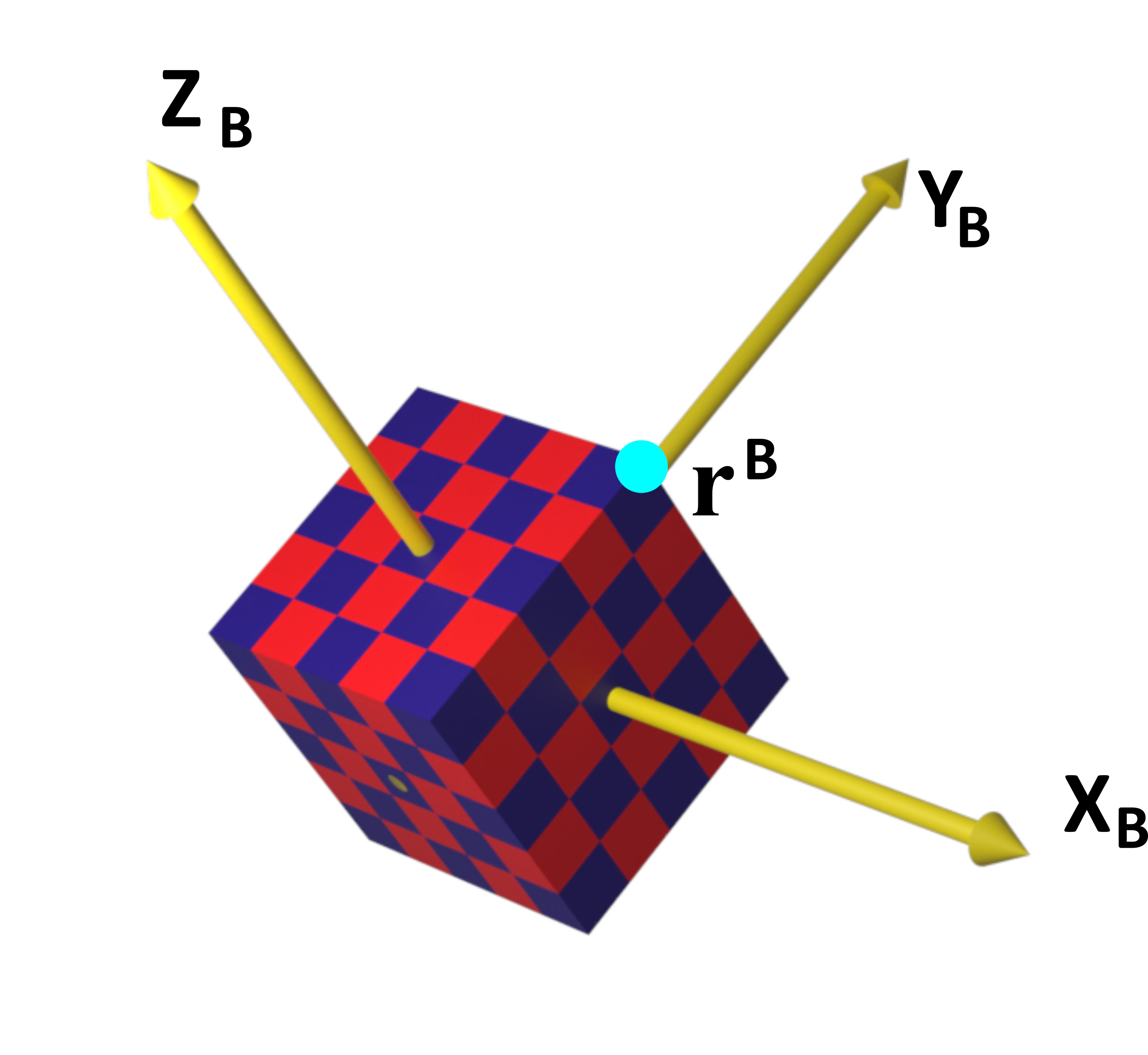
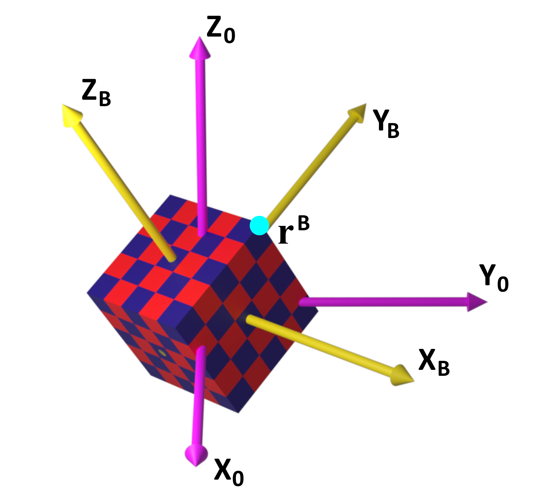
For example, let us assume that the 3D cube is a unit cube. Then, a vertex or a corner of the cube in the coordinate system has the following projections

(2)  

The point determined by this vector is shown in the figure below.

A similar notation is valid for , , and , that is

(3)  

We want to address the following problem. We are given the angles of rotation and and we are given the projections of the vector in the coordinate system . That is, we are given . We want to determine the coordinates of the vector in the coordinate system , that is, we want to determine the projections of .

Let us illustrate this problem with an example. Consider the figure shown below.

To solve this problem, we need to use rotation matrices that are explained in our previous tutorials, given here, here, and here. Let us now look at the rotation shown in Fig. 2.. By using the rotation matrices, we can represent the vector in the coordinate system by using this transformation

(4)  

where is the rotation matrix. The matrix is also denoted by . The notation is the classical notation for the rotation matrix that transforms the coordinate system into the coordinate system . Since the rotation is performed around the axis, according to our previous tutorial on the rotation matrices which can be found here, the rotation matrix has the following form

(5)  

Next, by using the same logic, from Fig. 2. above, we obtain

(6)  

where (or equivalently, ) is the rotation matrix transforming the coordinate system into the coordinate system . Since the rotation is performed with respect to the axis , according to our previous tutorial, which can be found here, the rotation matrix is defined by

(7)  

Finally, by using the same logic, from Fig. 2 above, we have

(8)  

where is the representation of the vector in the coordinate system , and (or equivalently, ) is the rotation matrix transforming the coordinate system into the coordinate system . Since the rotation is performed with respect to the axis , the rotation matrix is defined by

(9)  

By combining the equations (4), (6), and (8) we obtain

(10)  

The last expression can be written compactly as follows

(11)  

where

(12)  

The matrix is the direction cosine matrix. It transforms the projections of vectors from the coordinate system to projections of vectors in the coordinate system . In our previous tutorial, which can be found here, we explained the main properties of the direction cosine matrix. Next, let us find the explicit form of the matrix :

(13)  

where is the short notation for and is the short notation for .

The equation (11) solves our problem. The Python code given below is used to compute the direction cosine matrix :

# -*- coding: utf-8 -*-
"""
Demonstration of rotation matrices and
direction cosine matrix in Python 
by using the SymPy library 
- Symbolic Python Toolbox 
Author: Aleksandar Haber
"""

from sympy import * 

init_printing()

theta1=symbols('theta1')
theta2=symbols('theta2')
theta3=symbols('theta3')

Rtheta1=Matrix([[cos(theta1), -sin(theta1), 0],
                 [sin(theta1), cos(theta1),0],
                 [0, 0, 1]
                 ])

Rtheta2=Matrix([[1, 0, 0],
                 [0, cos(theta2), -sin(theta2)],
                 [0, sin(theta2), cos(theta2)]
                 ])

Rtheta3=Matrix([[cos(theta3), -sin(theta3), 0],
                 [sin(theta3), cos(theta3),0],
                 [0, 0, 1]
                 ])

# determine the direction cosine matrix
M=Rtheta1*Rtheta2*Rtheta3

# print(M)

# double check the orthogonality
simplify(M.T*M)

simplify(M.T*M -eye(3)) 

# generate the latex script
print_latex(M)