Transient Response of a Prototype Second-Order Dynamical System with Detailed Derivation Using Inverse Laplace Transform (damping, natural frequency, and damping ratio)

In this post, we explain how to analytically compute a transient response of a prototype second-order linear dynamical system. We start from a generic (prototypical) form of the second-order system, and we explain how to compute its step response (transient response) by using the inverse Laplace transform. The derivation and analysis presented in this post are very useful for understanding the transient response of linear dynamical systems and how different parameters, such as damping, natural frequency, etc. influence the transient response behavior. The YouTube video accompanying this post is given here

The prototype second-order system has the following form:

(1)  

where

• is the complex variable
• is the natural undamped frequency
• is the damping ratio

In this post, we derive the expression for the step response of the system (1). The step response is given by the following equation

(2)  

This equation can also be written as follows

(3)  

The general form of the second-order transfer function given by (1) is often used in control systems textbooks and articles. Moreover, many properties of the dynamical systems are often expressed in terms of the undamped natural frequency and the damping ratio . Consequently, before we proceed with the derivation of the step response of the second-order system (1), we relate the poles of this system with the natural undamped frequency and the damping ratio.

The poles of the dynamical system (1), are computed as follows:

(4)  

(5)  

where is the imaginary unit and

(6)  

These poles have a very useful graphical interpretation given in the figure below.

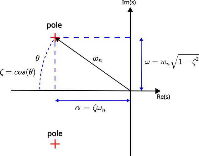
Here is an interpretation of Fig. 1:

• The natural undamped frequency is the distance from the pole to the origin.
• The damping ratio can be interpreted as the cosine of the angle .
• The parameter is called the damping factor or the damping constant.
• When , the system is critically damped. In this case, . This enables us to define the damping ratio as:
  

  (7)  

• The parameter is called the damped frequency or the conditional frequency.

In the sequel, we derive an analytical expression for the step response of the system (1). The output of the system can be represented as follows:

(8)  

Since we are interested in the step response, we assume . By substituting this expression in (8), we obtain

(9)  

We use partial fraction expansion to compute the response. The partial fraction expansion of (9) is given by

(10)  

We first need to determine the constants , , and , and after that, we can compute the inverse Laplace transform to compute the system response in the time domain. The partial fraction expansion and the cover method for computing it is explained in our previous post which can be found here. By applying the cover method, we obtain the value for the constant

(11)  

The constant is computed as follows

(12)  

Here, we used the following expression

(13)  

which originates from the following fact

(14)  

Going back to (12), we obtain

(15)  

Next, we substitute the expressions for and from (6) in (15), and as a result, we obtain

(16)  

Next, let us write the complex number in the polar form

(17)  

On the other hand, from Figure 1, we have that

(18)  

By substituting (18) in (17), we obtain

(19)  

Substituting (19) in (16), we obtain

(20)  

Next, we compute the constant by using the same strategy

(21)  

Next, by substituting (6) in (21), we obtain

(22)  

By using the previously explained polar transformation of complex numbers, we obtain

(23)  

Now, taking into account that , from (23), we obtain

(24)  

By using (11), (20), and (24), we can write (10) as follows

(25)  

Now, we need to find an inverse Laplace transform of (25). We need the following inverse Laplace transforms

(26)  

By using these inverse transforms, from (25}), we obtain

(27)  

Next, we use the following trigonometric identity

(28)  

for some angle . By using this expression in (27), we obtain

(29)  

Next, we use the following trigonometric expression

(30)  

By using this expression in (31), we obtain

(31)  

That is, the final expression is given by

(32)  

Using the procedure explained in the post that can be found here, we can also write the equation (32) as follows

(33)