Solve Inverse Kinematics Problem in MATLAB

In this post, we learn how to solve an inverse kinematics problem in MATLAB. In our previous post, which can be found here, we provided an introduction to the inverse kinematics problem. We explained how to analytically solve the inverse kinematics problem. However, in many cases it is either not possible to find the analytical solution or the analytical solution is too complex. In such cases, it is preferable to numerically approximate the solution. In this post and in the accompanying video we will explain how to compute the analytical solution. The YouTube video accompanying this post is given here

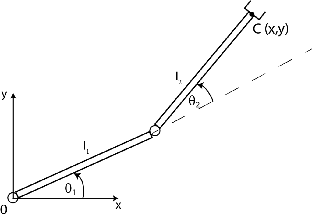
Consider a manipulator with two rotational degrees of freedom and shown in the figure below.

The inverse kinematics problem can be formulated as follows:

Given the coordinates x and y of the end-effector point C (world coordinates), compute the angles and (local joint coordinates).

In the statement of the inverse kinematics problem, it is assumed that the lengths of the robotic segments and are given.

From Figure 1, we have

(1)  

Now, for given and , and for given and , the equations (1) represent a system of nonlinear equations where unknown variables are and .

In the post given here, we explained how to solve a system of nonlinear equations in MATLAB. In this post, we follow the explained procedure. First, we transform the system (1) as follows

(2)  

First, we define a MATLAB function that describes the system (2)

function F=kinematics(theta,x,y,l1,l2)
F=[x-l1*cos(theta(1))-l2*cos(theta(1)+theta(2));
   y-l1*sin(theta(1))-l2*sin(theta(1)+theta(2))];
end

We save this function in the file called “kinematics.m”, and add the folder in which this function is saved to the MATLAB path.

This MATLAB function is called from the following MATLAB code

clear, pack, clc
% Possible algorithms 'trust-region-dogleg', 'trust-region', or 'levenberg-marquardt'
options = optimoptions(@fsolve,'Algorithm','trust-region','Display','iter','UseParallel',false,'OptimalityTolerance',1.0000e-8,'FunctionTolerance',1.0000e-12)

%% test cases
%x=0.8; y=0; l1=0.3;l2=0.5; % horizonal position, theta1=0 [deg], theta2=0 [deg]
x=0.4; y=0.4; l1=0.4;l2=0.4; % horizonal position, theta1=0 [deg], theta2=90 [deg]

% initial guess in degrees
% initialGuessDegrees=[10; 10]  % for 0-0
initialGuessDegrees=[20; 60]

% initial guess in radians
initialGuessRadians=initialGuessDegrees*(pi/180)

 
[solutionThetaRadians] = fsolve(@(theta)kinematics(theta,x,y,l1,l2),initialGuessRadians,options)
 
kinematics(solutionThetaRadians,x,y,l1,l2)

solutionThetaDegrees=solutionThetaRadians*(180/pi)

To solve the system of nonlinear equations, we need to specify and . This is done on code lines 6-7. We consider two test cases. In the first case, and . The second case is and . Then for these cases, we define initial guesses of and . To solve the system of nonlinear equations we need to specify the initial conditions. On code line 14, we transform initial guesses to radians. Code line 17 is used to solve the system of nonlinear equations. Code line 19 is used to verify the solution, by evaluating the right-hand side of (2). Code line 21 is used to transform the solution to degrees.

The test cases used in this tutorial, are explained in the figure given below.

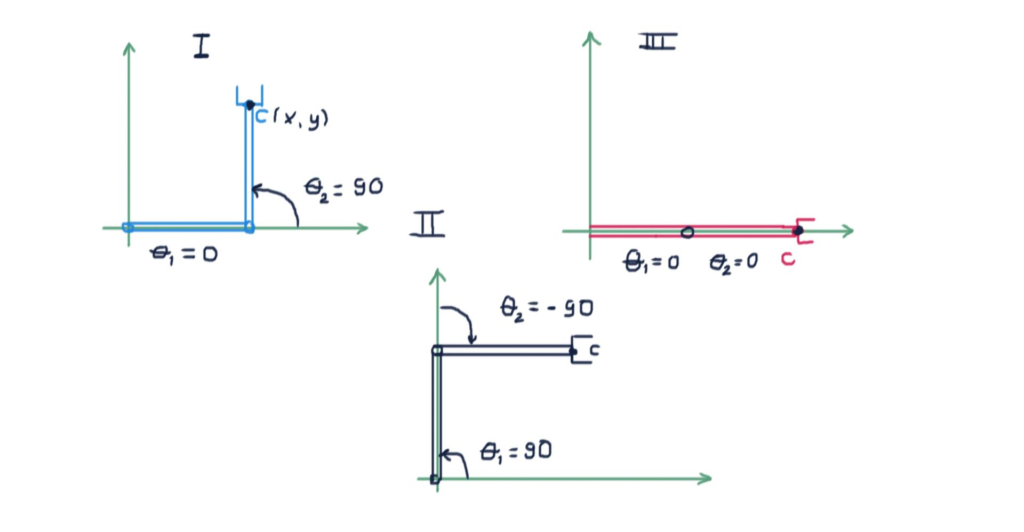
For an explanation of these test cases, see the youtube video.