In this Python tutorial, we will learn how to solve differential equations with time-varying inputs and coefficients in Python. We use the odeint() Python function. The GitHub page with all the codes is given here.
The YouTube tutorial accompanying this post is given below.

Test case – Nonlinear Pendulum
To explain the procedure for solving ordinary differential equations with time-varying inputs and coefficients, we need a test case. As a test case, we are using an example of a pendulum system shown in the Figure below.

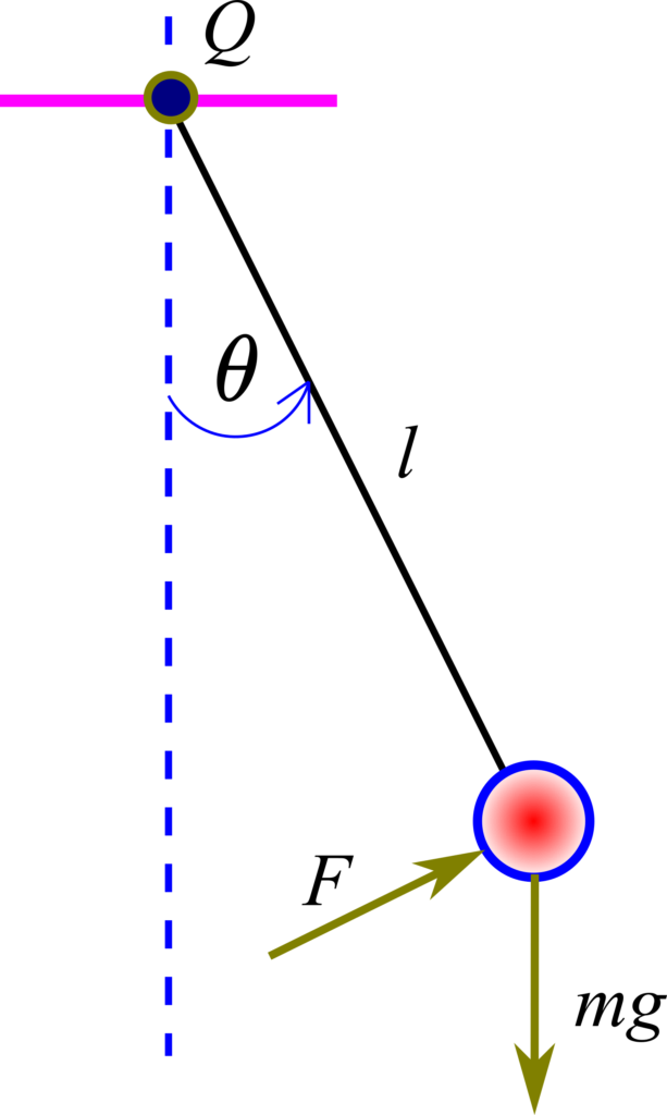
A ball (red color in the figure) with a mass of 


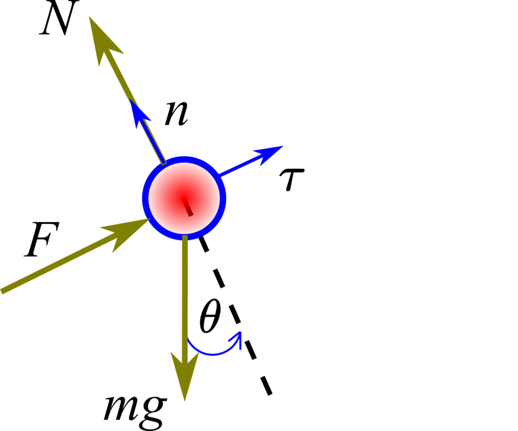
In the figure above, 


(1) 

where 


(2) 

where we assume that the force 


On the other hand, the tangential acceleration is given by
(3) 

where 


(4) 

From this equation, we obtain
(5) 

Let us write the ordinary differential equation (5) in the state-space form. This is necessary since Python’s solver needs a state-space form of differential equation in order to solve it.
First, we introduce the state-space variables
(6) 

By differentiating the last two equations, we obtain
(7) 

Consequently, the state-space model has the following form
(8) 

Python Numerical Solution
We compute the solution of the system (8), by using the odeint() function and interpolation. We are using the interpolation approach since we are assuming that the force F(t) is given at the discrete-time points. We can easily modify approach when the analytical form of the force
First, we need to import the necessary libraries and define the constants/parameters
import numpy as np
from scipy.integrate import odeint
import matplotlib.pyplot as plt

# define the constants
gConstant=9.81
lConstant=1
mConstant=5
Next, let us test interpolation in Python. The code presented in the sequel will interpolate values of a sinusoidal function at desired points that are not defined by a given set of discrete time instants and corresponding values of the sinusoidal function.
###############################################################################
# first, let us test the interpolation

timeArray=np.linspace(0,2*np.pi,100)
sinArray=np.sin(timeArray)
plt.plot(timeArray, sinArray)

# interpolate the values
np.interp((timeArray[9]+timeArray[10])/2,timeArray, sinArray)

# compare the interpolated values with sinArray[9] and sinArray[10]
# the interpolated value should be between these two values
###############################################################################
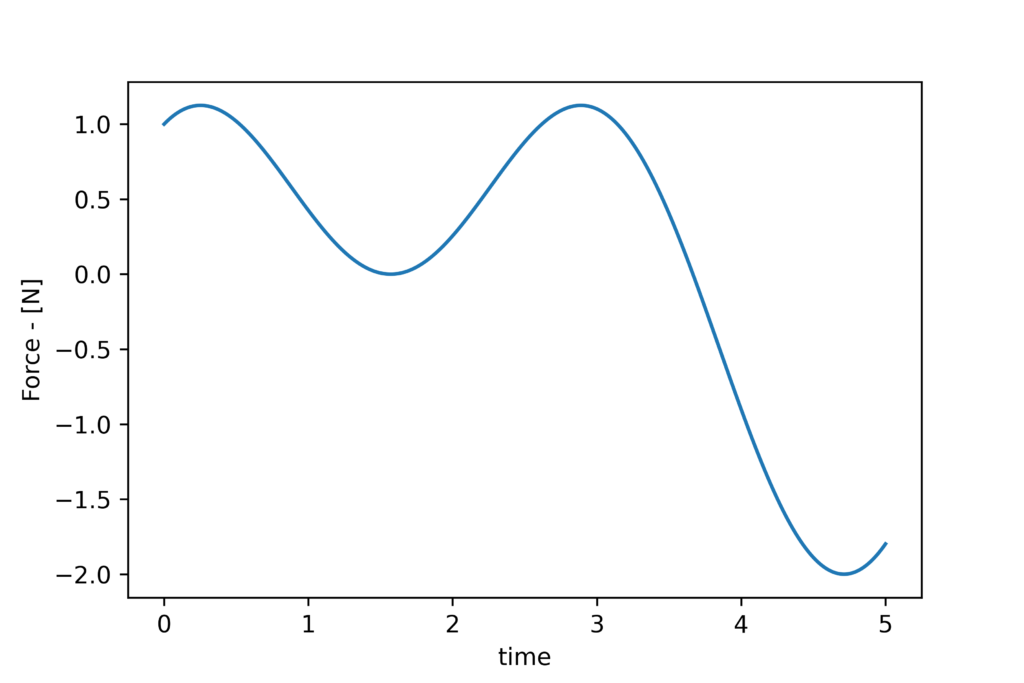
Now that we know how to interpolate the function values, we can proceed further. For illustration, we generate data points corresponding to an input force function that has the following analytical form
(9) 

This is achieved by using the following code
# now simulate the dynamics

startTime=0
endTime=5
timeSteps=1000

# simulation time array
# we will obtain the solution at the time points defined by
# the vector simulationTime
simulationTime=np.linspace(startTime,endTime,timeSteps)

# define the force input
forceInput = np.sin(simulationTime)+np.cos(2*simulationTime)
plt.plot(simulationTime, forceInput)
plt.xlabel('time')
plt.ylabel('Force - [N]')
plt.savefig('inputSequence.png',dpi=600)
plt.show()
The force function is shown in the figure below.

To simulate the differential equation, we need to define a function that evaluates the right-hand side of the model (8) for the current simulation time 

We do that by using the following Python code.
# this function defines the state-space model, that is, its right-hand side
# x is the state
# t is the current time - internal to solver
# timePoints - time points vector necessary for interpolation
# g,l,m constants provided by the user
# forceArray - time-varying input
def stateSpaceModel(x,t,timePoints,g,l,m,forceArray):
    # interpolate input force values
    # depending on the current time
    forceApplied=np.interp(t,timePoints, forceArray)
    # NOTE THAT IF YOU KNOW THE ANALYTICAL FORM OF THE INPUT FUNCTION
    # YOU CAN JUST WRITE THIS ANALYTICAL FORM AS A FUNCTION OF TIME
    # for example in our case, we can also write
    # forceApplied=np.sin(t)+np.cos(2*t)
    # and you do not need to specity forceArray as an input to the function
    # HOWEVER, IF YOU DO NOT KNOW THE ANALYTICAL FORM YOU HAVE TO USE OUR APPROACH
    # AND INTERPOLATE VALUES

    # right-side of the state equation
    dxdt=[x[1],-(g/l)*np.sin(x[0])+(1/(m*l))*forceApplied]
    return dxdt
This function accepts the following input parameters:
- “x” is a 2 by 1 vector (or a list) – this is the state vector at the time instant
- “t” is the current time that is varied by the solver
- “timePoints” is a vector or an array of time points that is used for interpolating the values of the input force
- “g, l, m” are parameters of the model
- “forceArray” is the vector of forces at the points “timePoints”
This function will interpolate the values of the force function for the current value of time “t”. Then, for such a value, and for the value of the current state it will evaluate the right-hand side of the state equation. Here it should be noted that we can easily modify this function to accept the analytic form of the function
We solve the problem by using the following code lines.
# define the initial state for simulation
# position and velocity
initialState=np.array([0,0])
# generate the state-space trajectory
solutionState=odeint(stateSpaceModel,initialState,simulationTime,args=(simulationTime,gConstant,lConstant,mConstant,forceInput))
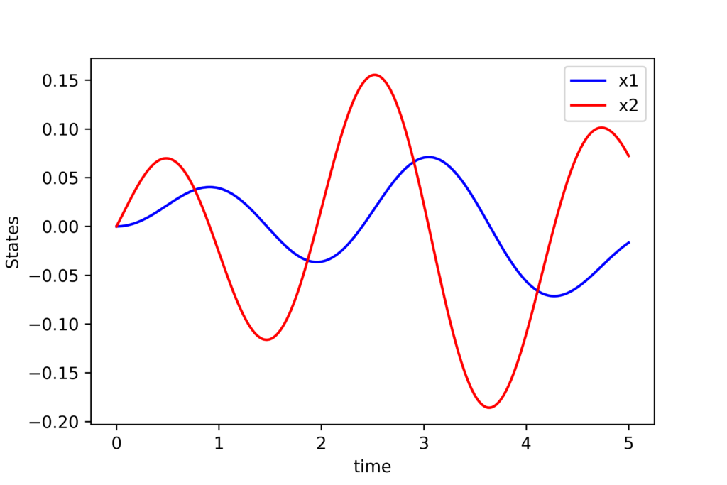
plt.plot(simulationTime, solutionState[:,0],'b',label='x1')
plt.plot(simulationTime, solutionState[:,1],'r',label='x2')
plt.xlabel('time')
plt.ylabel('States')
plt.legend()
plt.savefig('simulationResult.png',dpi=600)
plt.show()
First, we define the initial state. The initial state is defined by the vector “initialState”. We numerically solve the differential equation by using the function “odeint()”. The input arguments of this function are:
- “stateSpaceModel” – previously defined function that defines the right-hand side of the state-space model (8)
- “initialState” – previously defined initial state for solving the problem
- “simulationTime” – array of time steps at which the solution is computed
- “(simulationTime,gConstant,lConstant,mConstant,forceInput)” – this is a tuple that is passed as a set of parameters to the function. It consists of “simulationTime”, model parameters, and the array “forceInput” that together with “simulationTime” define the set of points that are used for interpolating the input force.
This code produces the graph shown below which presents the simulated state trajectories.