Solve Differential Equations Analytically Using MATLAB Symbolic Math Toolbox

In this lecture, we explain how to solve differential equations analytically using MATLAB Symbolic Math Toolbox. Furthermore, we explain how to plot a graph of the derived analytical solution. The YouTube video accompanying this post is given below.

Consider the following linear ordinary differential equation

(1)  

where is the variable we want to solve for,, , , and are constants, and is the specified function of time. For example, as we have explained in our previous lecture, the equation (1) can represent a mass-spring-damper system that is driven by the force .

Our goal is to derive an analytical solution of (1) using MATLAB Symbolic Toolbox.

The first step is to define the symbolic variables. This can be done as follows.

syms d(t) kd ks mass Force(t)

Here we specify that , , , and are symbolic variables, that correspond respectively to the variables and constants , , , and in (2). Here it should be emphasized that it is important to define and as functions of time. This is achieved by typing and .

The next step is to define the first and second derivatives of . This can be done as follows.

ddot_d=diff(d,t,2)
dot_d=diff(d,t,1)

Let us assume that the variable is equal to . For such a choice of the right-hand side of Eq. (2), we define the differential equation as follows

dynamics_equation=mass*ddot_d+kd*dot_d+ks*d == sin(t)

This code is self-explanatory. To be able to solve the differential equation, we need to specify the initial conditions for and (position and velocity). This can be done as follows.

initial_conditions=[d(0)==1, dot_d(0)==0]

We solve the equation by executing the following line of code.

solution=dsolve(dynamics_equation,initial_conditions)

We can also simplify the solution by executing the following line of code.

solution2=simplify(solution)

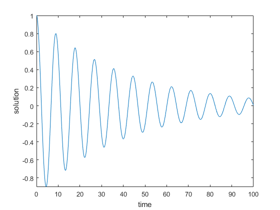
The next step is to plot the solution. In order to plot the solution, we need to select the values of the parameters , , and . This can be done by executing the following line of code.

solution3=subs(solution2,{mass,ks,kd},{2,1,0.1})

That is, we choose , , and . We can also simplify or expand the substituted solution as follows.

solution4=simplify(solution3)

solution5=expand(solution3)

Finally, the substituted solution can be plotted by executing the following code lines.

plotting_interval=[0,100]

fplot(solution4,plotting_interval)
xlabel('time')
ylabel('solution')

First, we choose the plotting interval, and then similarly to the MATLAB function plot(), we can use the function to plot the solution. The result is shown in the figure below.

Finally, let us verify that this approach produces accurate results. The idea is to compare this approach with another approach for computing the analytical solution. The two approaches should produce results that match. The approach that is used for comparison is based on the Laplace transform. We perform the tests using the following differential equation

(2)  

where is time variable. Let us assume that initial conditions are and . Let us apply the Laplace transform to equation (2). Let be the Laplace transform of . By applying the Laplace transform to (2), we obtain

(3)  

Taking into account that and , and by transforming the expression (3), we obtain

(4)  

By applying the inverse Laplace transform to (4), we can obtain as function of . We use MATLAB to compute the inverse Laplace transform. The inverse Laplace transform can be computed by executing the following code lines

syms s 

Ds=s/(s^2+4)+(1/(s^2))*(1/(s^2+4))

inverseLaplace=ilaplace(Ds)
simplify(inverseLaplace)

The result is

t/4 + cos(2t) – sin(2t)/8

Let us now compute the solution by analytically solving the equation (2). The code for solving this equation is given below.

clear, pack, clc
syms d(t) 

ddot_d=diff(d,t,2)
dot_d=diff(d,t,1)

dynamics_equation=ddot_d+4*d == t

initial_conditions=[d(0)==1, dot_d(0)==0]

solution=dsolve(dynamics_equation,initial_conditions)

solution2=simplify(solution)

The results is

t/4 + cos(2t) – sin(2t)/8

We can see that the two approaches produce the identical results.