Pole Placement to Meet the Requirements on Desired Overshoot and Rise Time – Control Engineering Tutorials

In this control engineering tutorial, we explain how to design a state feedback control law such that the poles of the closed-loop system are placed at the appropriate locations that guarantee that the step response meets the desired specifications. The important technique presented in this tutorial is widely used in the control system engineering practice. The YouTube tutorial accompanying this post is given below.

Problem Formulation and Solution

We explain this technique by using a particular example that is presented in the sequel. Consider the following open-loop transfer function:

(1)  

We need to design a state feedback control system such that the following requirements are satisfied

1.) The rise time should not be larger than 1 second.
2.) The overshoot should not be larger than 10 percent.

Solution:

The first step is to develop a state-space model corresponding to the system (1). To develop the state-space model, we use the controllable canonical form explained in our previous tutorial. We use this approach since the controllable canonical form enables us to quickly compute the characteristic polynomial of the closed-loop system. We can also use other methods for pole placement, such as MATLAB’s function place().

First, we expand the transfer function:

(2)  

We can observe that the polynomials in the numerator and denominator are

(3)  

Then, the controllable canonical form is given below

(4)  

Our goal is to design a feedback control law

(5)  

such that the poles of the closed-loop system are placed at proper locations that we need to determine in the sequel. Later on, we will modify this control law to introduce a reference signal and an additional gain to ensure that step responses are properly tracked.

To determine the pole locations, we need to recall the basic pole parametrization in terms of the damping ratio and natural undamped frequency . The figure below shows the parametrization idea.

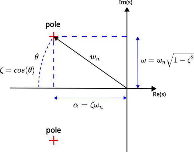
The poles are parametrized by

(6)  

Although our system is of the third order, for selection of the parameters and we use a second order approximation of the dynamics. This approximation is justified for dominant poles. That is, it approximates the dynamics of the dominant poles fairly well, as long as the third pole is placed far away from these dominant poles. The second-order prototype system is parametrized by

(7)  

For such a system, we can relate overshoot and rise time with the damping ratio and natural undamped frequency . We can use the formulas given in Chapter 7 (pages 334,335, and 336) of “Automatic Control Systems” by Benjamin Kuo. The maximum overshoot is given by the following formula:

(8)  

where is the maximum overshoot. On the other hand, the rise time is given by the following equation

(9)  

From (8), we can find by using the desired specification of the maximum overshoot. Then, by using the desired specifications on the rise time and the computed , we can determine . Once we determine and , we substitute them in (6), to determine the pole locations that approximately produce the desired transient response.

From (8), we have

(10)  

By substituting the desired in the last equation, we obtain the value for :

(11)  

Since for larger values of we obtain smaller overshoots, we round this computed value of to

(12)  

On the other hand, from (9), we have

(13)  

By substituting this value in (12), we obtain the value of

(14)  

Since larger values of produce smaller rise time, we round this number to obtain the final value for

(15)  

Having these values, and by using (6) we can design the closed loop poles:

(16)  

We place the third pole relatively far away from these poles. We choose a real third pole

(17)  

The desired closed-loop characteristic polynomial has the following form

(18)  

This is our target characteristic polynomial that will guarantee the desired system transient behavior. On the other hand, let us consider the feedback control system obtained by substituting the feedback (5) in (4):

(19)  

We have

(20)  

We can observe that the closed-loop matrix is the controllable canonical form, and consequently, we can immediately write the closed-loop characteristic polynomial

(21)  

This parametrized polynomial should be equal to (18), that is,

(22)  

Two polynomials are equal if their coefficients are equal, consequently, we have

(23)  

That is,

(24)  

These coefficients of the feedback control matrix should guarantee the desired transient response characteristics. The final step is to add a reference signal to the control input.

To add the reference signal, we need to make the following analysis. Consider the system

(25)  

Let us assume that there exist a constant that produces a steady-state output and steady state . Then, , , and satisfy

(26)  

where in the steady state. By subtracting the state equations of the state space models (25) and (26), we obtain

(27)  

where , and . Since

(28)  

We have that (27) can be written as follows

(29)  

Here it should be noted that this system has the same state-space matrices as the original system (25). That is the matrices computed for such a system and for the original system are identical. Consequently, we can use the matrix for the original system to assign the poles to this system. The feedback control law will have the following form

(30)  

By expanding the last equation, we obtain

(31)  

Now, let us assume that the reference signal (desired constant signal that we want to follow) satisfies these equations

(32)  

where is a scalar and is a column vector that we want to determine. The equation (32) has a physical explanation. If the reference signal is constant, and the system is asymptotically stable, then, as the time approaches infinity the steady-state of the system will be reached. This means that there exist a linear relationship between and , and the coefficient of the linear relationship is precisely the vector . The scalar is just a scaling of the reference signal. On the other hand, for precise following of the reference signal in the steady-state, the following equations should be satisfied

(33)  

These equations are obtained by substituting (32) and in (26). From (33), we obtain by eliminating

(34)  

or

(35)  

We can solve these equations to compute the gains and , the solution is

(36)  

By using the computed values and by substituting (32) in (31), we obtain the final control law

(37)  

By substituting this control law in the state-space model (25), we obtain the final regulated system with the reference input

(38)  

The system (38) is regulated in the sense that it satisfies the desired transient characteristics and it follows the step signal .

The MATLAB code is shown below.

clear
% overshoot
Mos=10
MlogSq=(log(Mos/100))^2
% damping ratio
zeta=sqrt(MlogSq/(pi^2+MlogSq))
% rise time
tr=1;
% natural undamped frequency
omegaN=(1-0.4167*zeta+2.917*zeta^2)/tr;
% real part
realPart=omegaN*zeta;
% imaginary part
imaginaryPart=omegaN*sqrt(1-zeta^2);
% third pole
c=-6;
% closed loop polynomial
fcl=[1 -(c+2*(-realPart)) (2*(-realPart)*c+(-realPart)^2+(-imaginaryPart)^2) -c*((-imaginaryPart)^2+(-realPart)^2)]
roots(fcl)
realPart
imaginaryPart

A=[-4 0 0; 1 0 0; 0 1 0]; B=[1; 0; 0]; C=[0 0 1];
matrix1=[A, B; C, 0]; leftSide=[0;0;0; 1];
gainMatrix=inv(matrix1)*leftSide;

% this the feedback gain matrix
Kmatrix=[4.0963, 15.7215, 18.8623];
% closed loop matrix
Acl=A-B*Kmatrix;
% check the eigenvalues
eig(Acl)
% B matrix for the reference signal
Br=gainMatrix(4)+Kmatrix*gainMatrix(1:3);
Bcl=B*Br;
ssCl=ss(Acl,Bcl,C,[]);

step(ssCl)
tf(ssCl)

The computed closed-loop transfer function is

(39)  

The step response of the closed-loop function (step reference signal ) is shown in the figure below. This figure shows the rise time.

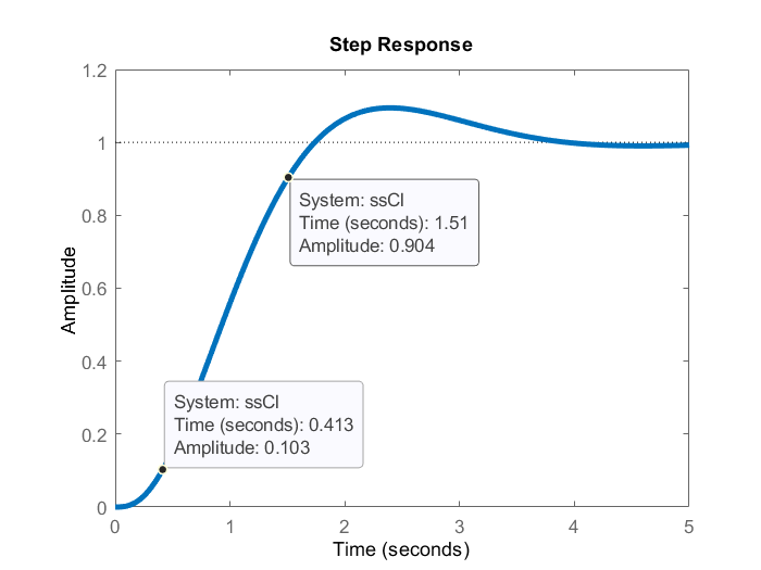
Figure 3 below shows the overshoot value of the same step response.

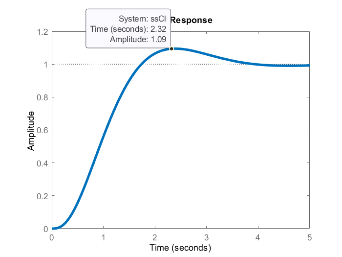
From figures 2 and 3, we can observe that the desired transient response specifications are achieved by placing the poles at the proper locations.