In this control system tutorial, we explain how to develop a controller by using a pole-placement method. The controller includes an integral control action to eliminate steady-state errors. We explain how to model and simulate this controller in Simulink and MATLAB. The YouTube tutorial is given below. In our next tutorial, whose link is given here, we explain how to model the Linear Quadratic Regulator (LQR) controller in Simulink.

As a test case, we consider the mass-spring-damper system shown in the figure below.

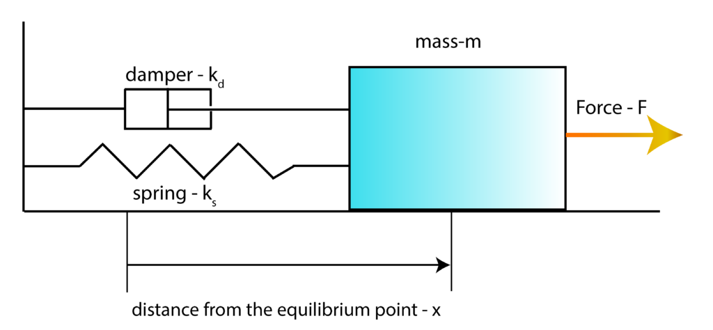
This model is thoroughly explained in our previous tutorial which can be found here. The distance from the equilibrium point is denoted by 


(1) 

The resulting state-space model has the following form:
(2) 

where
(3) 

Our goal is to design a controller that will make the output 


(4) 

Then, the goal of the controller is to decrease the control error as close as possible to zero.
The basic controller based on pole placement or Linear Quadratic Regulator (LQR) can be used to steer the system to the zero equilibrium point. That is, these controllers can be used to steer the system’s state to zero state 

We add an integrator by augmenting our original state-space model, with the state of the integral controller. Let us introduce a new variable 

(5) 

By taking the first derivative of (5), we obtain
(6) 

By substituting the output equation of the state-space model (2) in (6), we obtain
(7) 

By combining the state equation of the model (2) with the integral controller (7), we obtain
(8) 

The last two equations can be written in the compact form
(9) 

The last equation can be written compactly as follows
(10) 

where
(11) 

In this tutorial, we assume that the state vector of the augmented system 

(12) 

By partitioning 

(13) 

and by using the definition of
(14) 

By using (5), the last equation can be written as follows
(15) 

We can clearly observe that the controller explicitly takes into account the integral of the control error. To develop a Simulink model and simulate it, we need to create a block diagram of the system and the controller. The block diagram is given below.

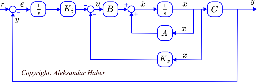
The MATLAB code is given below.
ks=1
kd=0.1
m=10

A=[0 1; -ks/m -kd/m];
B=[0; 1/m];
C=[1 0]
D=[0]

% compute the open loop poles
openLoopPoles=eig(A)

% form the augmented system
Aa=[A [0; 0]; -C 0]
Ba=[B;0]

% set the desired closed-loop pole locations
desiredClosedPoles=[-2+0.2i; -2-0.2i;-3]

% use the place command to place the closed loop poles at the desired
% locations
K=place(Aa,Ba,desiredClosedPoles)
% check the closed loop poles
eig(Aa-Ba*K)
% extract feedback matrices

Kx=K(:,1:2)
Ki=K(3)
This code will calculate the feedback control matrix 


