In this control engineering and control theory tutorial, we explain how to implement a sliding mode controller for a nonlinear system in MATLAB and Simulink. We mainly focus on the implementation and we briefly discuss the theory behind the sliding mode control algorithm. As a demonstration and as a proof of the implementation principle, we consider a nonlinear pendulum system. The YouTube tutorial is given below.

Sliding Mode Control of Nonlinear Pendulum Model
The pendulum system is shown below.

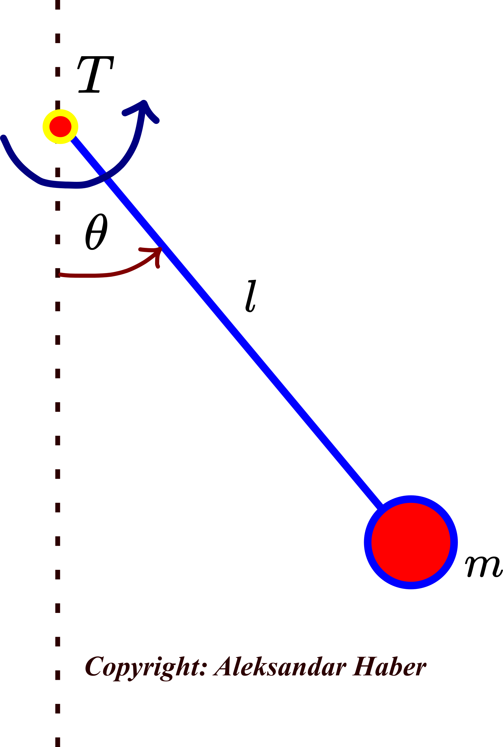
The mass of the ball is 


By using Newton’s second law, we obtain a differential equation describing the dynamics of the pendulum system
(1) 

Next, we introduce the following notation
(2) 

Consequently, the model looks like this
(3) 

The control objective is to design a controller and a sequence of control inputs 


We solve this problem by using the sliding mode controller. First, we introduce the tracking error 

(4) 

The first and second derivatives of the tracking error are defined below
(5) 

Secondly, we define the switching function (sliding function) as follows
(6) 

where 
The sliding mode control is computed by using the following equation:
(7) 

where 


(8) 

then, the controller achieves sliding mode and sliding motion. That is, the equation (8) defines the minimal value of the parameter
We need to show the following
(9) 

where 
First, let us take the first derivative of the switching function 

(10) 
On the other hand, by substituting the second equation from (5) (the second derivative of the tracking error) in (10), we obtain
(11) 

Next, by substituting the dynamics (3) in (11), we obtain
(12) 

Let us now substitute the control law (7) in (12). As a result, we obtain
(13) 

Next, by multiplying the last equation by
(14) 

Next, we use the following two equations:
(15) 

The last equation follows from the fact that the 


(16) 

From the last equation, we see that if
(17) 

or equivalently
(18) 
Then, the reachability condition is satisfied with 

(19) 
MATLAB and Simulink Implementation of Sliding Mode Control Algorithm
First of all, we create a MATLAB script that defines the model parameters.
% system parameters
g=9.81;
m=5;
l=1;
a=g/l;
b=1/(m*(l^2));
c=3;
k=2*a;

theta0=pi/6;
dtheta0=0.1;
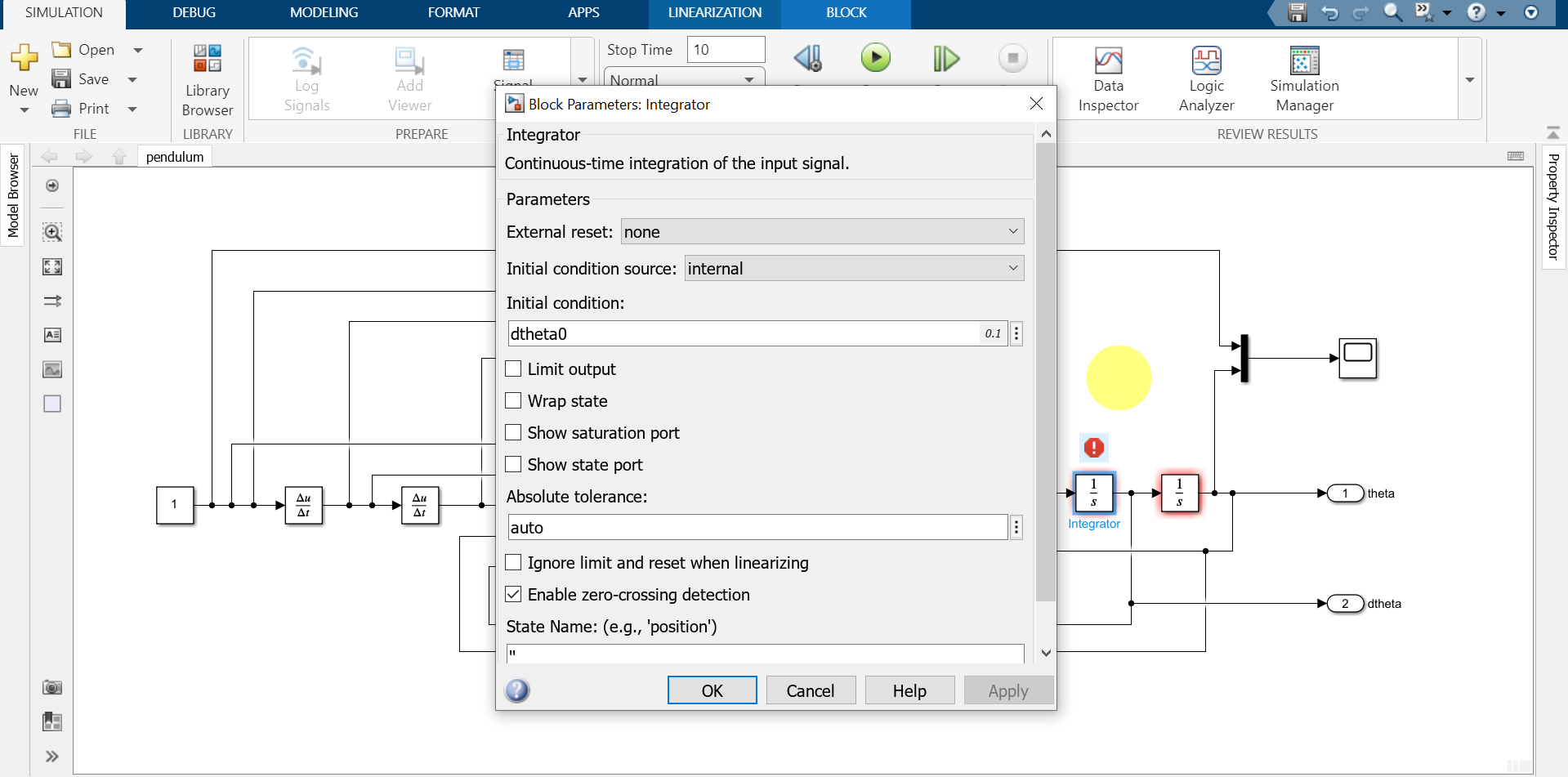
The last two parameters called “theta0” and “dtheta0” are initial conditions for simulating the dynamics. The Simulink block diagram is shown below.

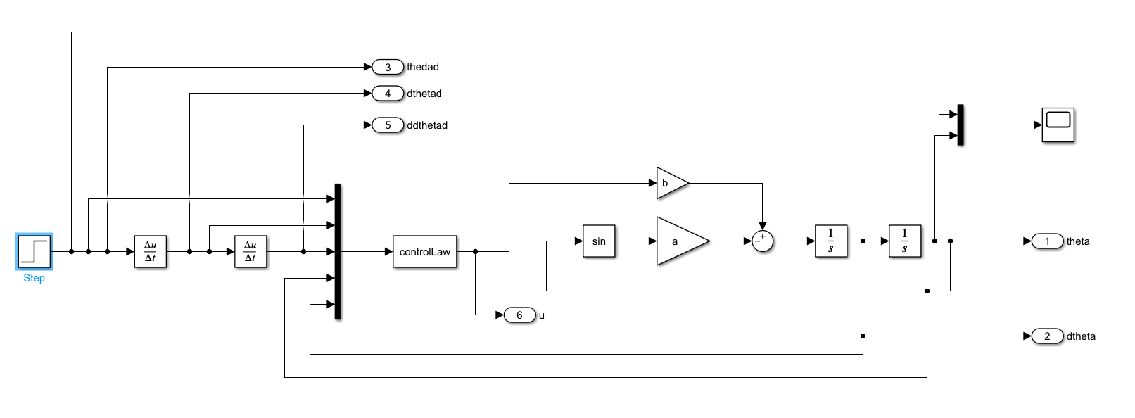
The dynamics is modeled by using the sin, two gain (a and b), sum, and two integrator blocks. The initial conditions are specified in the integrator blocks

The reference (desired) trajectory is a step signal. We also compute the first and second derivatives of the reference trajectory. We use the Mux block to group all the signals in a vector. This vector is passed to the MATLAB s-function block that implements the control law. The m-script called “controlLaw.m” implements the control law:
function [sys,x0,str,ts,simStateCompliance] = controlLaw(t,x,u,flag,b,k,c)
switch flag,

  case 0,
    [sys,x0,str,ts,simStateCompliance]=mdlInitializeSizes;
  case 1,
    sys=mdlDerivatives(t,x,u);

  case 2,
    sys=mdlUpdate(t,x,u);

  case 3,
    sys=mdlOutputs(t,x,u,b,k,c);

  case 4,
    sys=mdlGetTimeOfNextVarHit(t,x,u);

  case 9,
    sys=mdlTerminate(t,x,u);

   otherwise
    DAStudio.error('Simulink:blocks:unhandledFlag', num2str(flag));

end


function [sys,x0,str,ts,simStateCompliance]=mdlInitializeSizes

sizes = simsizes;

sizes.NumContStates  = 0;
sizes.NumDiscStates  = 0;
sizes.NumOutputs     = 1;
sizes.NumInputs      = 5;
sizes.DirFeedthrough = 1;
sizes.NumSampleTimes = 1;   % at least one sample time is needed

sys = simsizes(sizes);

x0  = [];

str = [];

ts  = [0 0];

simStateCompliance = 'UnknownSimState';

function sys=mdlDerivatives(t,x,u)

sys = [];

function sys=mdlUpdate(t,x,u)

sys = [];

function sys=mdlOutputs(t,x,u,b,k,c)
% u(1) - theta_d reference trajectory (desired trajectory)
% u(2) - derivative of theta_d
% u(3) - second derivative of theta_d
% u(4) - theta
% u(5) - derivative of theta

error=u(1)-u(4);
derror=u(2)-u(5);

sigma=c*error+derror;

control=(1/b)*(c*derror+u(3)+k*sign(sigma));

sys = control;


function sys=mdlGetTimeOfNextVarHit(t,x,u)

sampleTime = 1;    %  Example, set the next hit to be one second later.
sys = t + sampleTime;


function sys=mdlTerminate(t,x,u)

sys = [];
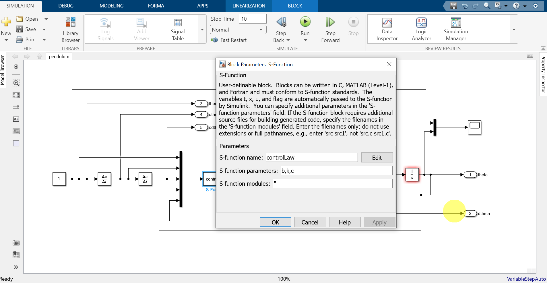
The parameters of the s-function block are shown below.

We use the outport blocks to export all the variables to the MATLAB workspace. The code below is used to plot the results once the variables are exported to the MATLAB workspace.
<pre class="wp-block-syntaxhighlighter-code">
% theta
theta=out.yout{1}.Values.Data;
% derivative of theta
dtheta=out.yout{2}.Values.Data;
% thetad - desired value
thetad=out.yout{3}.Values.Data;
% first derivative of thetad
dthetad=out.yout{4}.Values.Data;
% second derivative of thetad
ddthetad=out.yout{5}.Values.Data;
% control input
u=out.yout{6}.Values.Data;
% error
e=thetad-theta;
% first derivative of error
de=dthetad-dtheta;
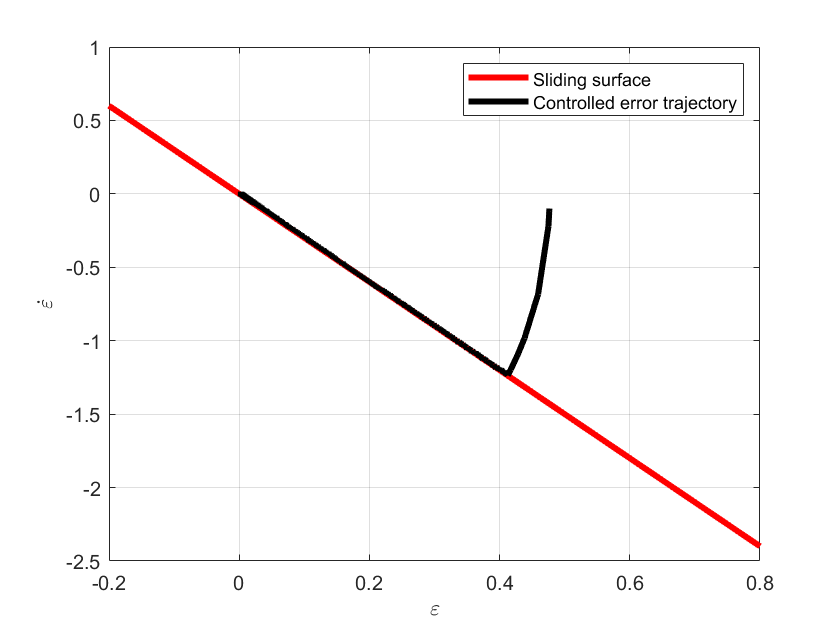
% define the sigma line
xLine=-0.2:0.01:0.8;
yLine=-c*xLine;
% switching function
sigma=c*e+de;
figure(1)
hold on
grid
box
plot(xLine,yLine,'r',LineWidth=3)
plot(e,de,'k',LineWidth=3)
xlabel('<img src="https://aleksandarhaber.com/wp-content/ql-cache/quicklatex.com-305d0239fb65087cbb5b6ccd24cec1ce_l3.png" class="ql-img-inline-formula quicklatex-auto-format" alt="{\varepsilon }" title="Rendered by QuickLaTeX.com" height="8" width="8" style="vertical-align: 0px;"/>','interpreter','latex','FontWeight','bold')
ylabel('<img src="https://aleksandarhaber.com/wp-content/ql-cache/quicklatex.com-d2c09514f46156d1d7aa802280b8bbbe_l3.png" class="ql-img-inline-formula quicklatex-auto-format" alt="{\dot{\varepsilon}}" title="Rendered by QuickLaTeX.com" height="12" width="8" style="vertical-align: 0px;"/>','interpreter','latex','FontWeight','bold')
legend('Sliding surface','Controlled error trajectory')
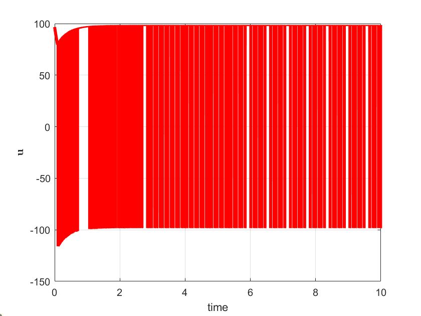
figure(2)
hold on
grid
box
plot(out.tout,u,'r',LineWidth=3)
xlabel('time')
ylabel('<img src="https://aleksandarhaber.com/wp-content/ql-cache/quicklatex.com-b1eede20187d03f368a6ce744e1155f2_l3.png" class="ql-img-inline-formula quicklatex-auto-format" alt="{\mathbf{u}}" title="Rendered by QuickLaTeX.com" height="8" width="11" style="vertical-align: 0px;"/>','interpreter','latex','FontWeight','bold')
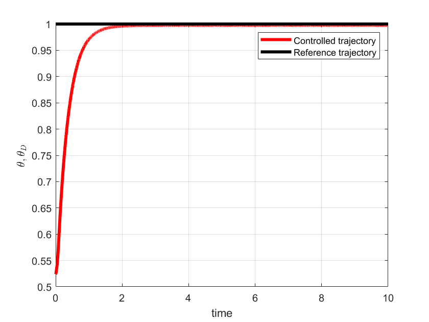
figure(3)
hold on
grid
box
plot(out.tout,theta,'r',LineWidth=3)
plot(out.tout,thetad,'k',LineWidth=3)
xlabel('time')
ylabel('<img src="https://aleksandarhaber.com/wp-content/ql-cache/quicklatex.com-712c27de1b43423e8d2f7caccf11250d_l3.png" class="ql-img-inline-formula quicklatex-auto-format" alt="{\theta},{\theta_{D}}" title="Rendered by QuickLaTeX.com" height="16" width="36" style="vertical-align: -4px;"/>','interpreter','latex','FontWeight','bold')
legend('Controlled trajectory','Reference trajectory')
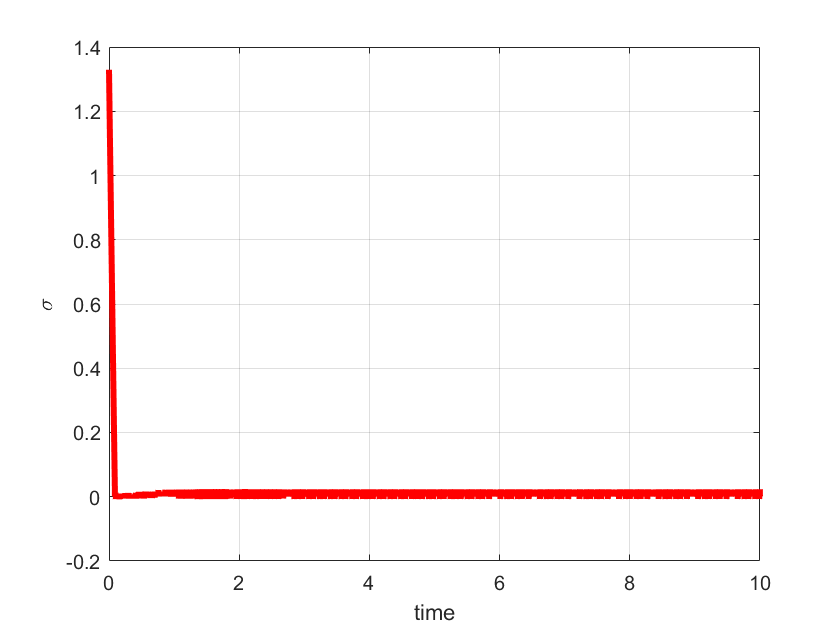
figure(4)
hold on
grid
box
plot(out.tout,sigma,'r',LineWidth=3)
xlabel('time')
ylabel('<img src="https://aleksandarhaber.com/wp-content/ql-cache/quicklatex.com-1c9cc40f96a1492e298e7da85a2c1692_l3.png" class="ql-img-inline-formula quicklatex-auto-format" alt="\sigma" title="Rendered by QuickLaTeX.com" height="8" width="11" style="vertical-align: 0px;"/>','interpreter','latex','FontWeight','bold')
</pre>
The results are shown below.