Limitations of Proportional Control – Why We Need an Integrator in the Control Loop – Control Engineering Lecture

In this control engineering and control theory tutorial, by using an example, we explain the following important facts about proportional control

1. Without an integrator in the loop (an integrator can come from the plant or the controller), a proportional controller algorithm usually cannot achieve perfect set-point tracking. That is, a simple proportional controller without an integrator in the loop cannot eliminate a steady-state tracking error.
2. We can improve the performance of the proportional control algorithm by increasing the proportional control gain. This leads to the high-gain feedback control principle. However, high proportional control gain might have several negative effects.
3. The limitations of the simple proportional control imply that we need an integrator or an integral control action in the loop.

The example presented in this tutorial is very important for learning control engineering and for preparing control engineering interviews.

Example 1: Proportional Control of First Order System

Problem 1: Consider the control structure given in the figure below.

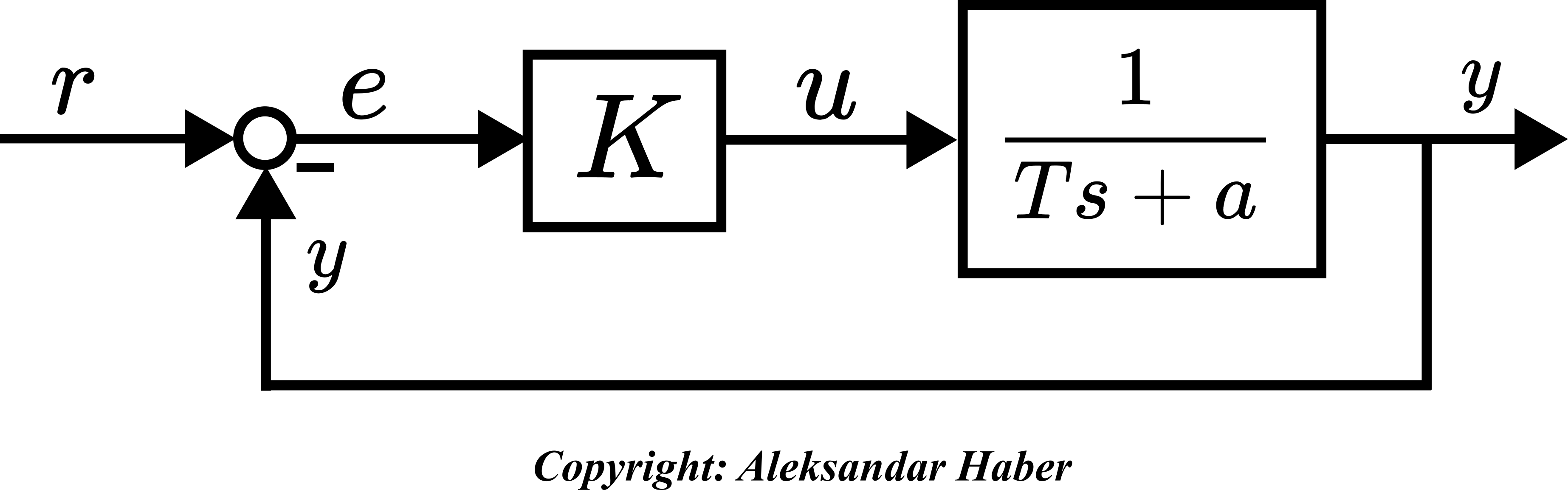
In the figure above, is the output of the system, is the control reference (set point), is the control input, is a proportional control gain, and and are arbitrary constants defining the transfer function of the plant:

(1)  

• Assume that the set point is a unit step signal. Is it possible to design the proportional control gain such that the steady state tracking error is equal to ?
• If NOT, how can we design the proportional control gain such that the steady-state tracking error is minimized?
• How do the model parameters and influence the steady-state error and our ability to control the system by using the proportional controller?

Solution:

The solution to this problem is to first derive the transfer function of the closed-loop system. From the figure above, we have

(2)  

where , , , , are the Laplace transform of the time domain signals , , , and . The closed-loop transfer function is

(3)  

From the third and second equations in (2), we have

(4)  

By substituting this equation in the first equation of (2), we obtain

(5)  

From the last equation, we have

(6)  

From the last equation in (6), we obtain the closed loop transfer function

(7)  

From the last equation, we obtain

(8)  

The unit step signal is . The Laplace transform of the unit step signal is

(9)  

By substituting (9) in (8), we obtain

(10)  

Let us compute the steady-state value of the output in the time domain. By using the final value theorem, we have

(11)  

By substituting (10) in (11), we obtain

(12)  

The steady-state error is given by

(13)  

The steady-state error is given by

(14)  

We can observe the following

• The proportional controller cannot achieve zero steady-state error.
• We can minimize the steady-state tracking error by selecting a large value of the gain . This leads to the high-gain feedback controller.
• We can observe that the parameter does not influence the value of the steady-state error.

Let us now investigate the influence of the parameter on the value of the steady-state tracking error. Let us assume that is constant, and let us compute the first derivative of with respect to . As a result, we have

(15)  

We can observe that the first derivative is positive. This means that the steady-state error increases with the increase of . All this implies that if has a small positive value ( is positive), then the steady-state error is close to zero if the proportional control gain is much larger than . When is close to zero, then the dynamics of the plant is slow. This means that we can effectively control very slow first-order systems with proportional control.

To achieve a zero value of the steady-state tracking error, either a controller or the plan need to contain an integrator. This will be explained in our next tutorial given here.