Example of Designing a Phase Lead Controller (Compensator) in MATLAB

In our previous post, which can be found here, we derived the main equations of the phase lead controller. Furthermore, in the same post, we summarized a procedure for designing the phase lead controller. In this post, we explain how this procedure can be used to design the parameters of the phase lead controller. The YouTube tutorial accompanying this tutorial is given below.

Problem

Consider the following open-loop system:

(1)  

Design the lead compensator such that the phase margin of the compensated system is at least 50 degrees.

Summary of the Design Procedure for the Phase Lead Compensator

Design specification and goal: Achieve the Phase Margin (PM) of the compensated system that is larger or equal to the minimum desired value of the PM. Design the parameters and of the lead compensator

(2)  

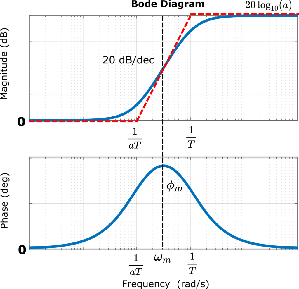
The Bode plot of the phase lead compensator is shown in the figure below.

PROCEDURE 1:

Step 1: Plot the Bode plot of the uncompensated system. Read the PM of the uncompensated system. On the basis of the PM of the uncompensated system and on the basis of the minimum desired PM, calculate the necessary value of (maximum phase of the lead compensator), as the difference between the minimum desired PM and the PM of the uncompensated system. That is, is the value of phase that needs to be added to the PM of the uncompensated system. Optionally, add a few degrees to this difference.

Step 2: For calculated , determine the parameter of the compensator by using the following formula

(3)  

Step 3: Select (frequency of the phase lead compensator that produces the maximum phase of the compensator) as the frequency where the gain of the uncompensated system is equal to . This will ensure that the gain cross-over frequency of the compensated system is approximately at .

Step 4: Select the parameter as

(4)  

Step 5: Plot the Bode plot, and check if the design specifications are met. If they are met, then we have designed the filter parameters and . If not, increase the previously computed value of , and repeat the steps 2, 3, 4, and 5.

Solution

Here, we present the solution of the problem. The MATLAB codes are given after each graph.

STEP 1: The bode plot of the open-loop system is given below.

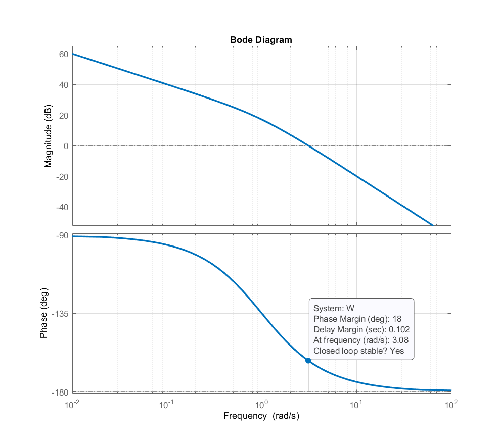
We can observe that the phase margin of the open-loop uncompensated system is degrees at the gain cross-over frequency of rad/s. Consequently, since the desired phase margin of the compensated system is 50 degrees, we have that the maximal phase of the lead compensator is

(5)  

Here, it is also instructive to plot the step response of the closed-loop system without the compensator. The step response of the closed-loop system is given below.

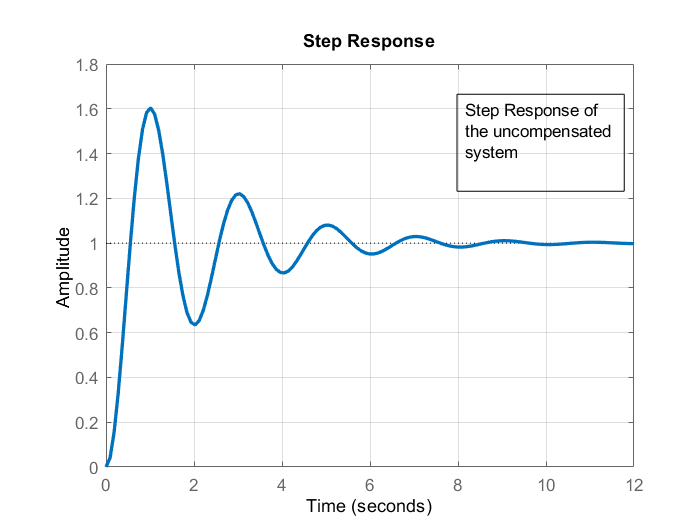
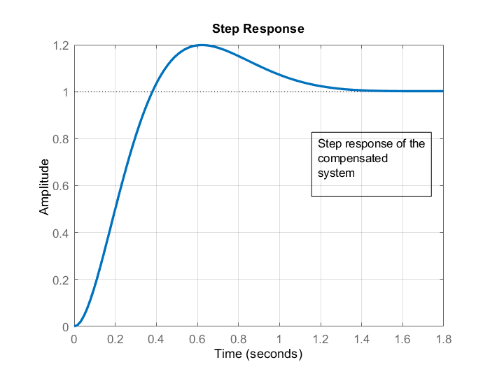
From Fig. 3., we can observe that the main issue with the step response of the closed loop of the uncompensated system is the large damping ratio. By increasing the phase margin, we will decrease the damping without affecting the steady-state characteristics.

We used the following MATLAB code lines to generate these plots

W=tf(10,[1 1 0])
figure(1)
bode(W)
Wfeedback=feedback(W,1)
figure(2)
step(Wfeedback)

STEP 2: We use the following formula to determine the parameter

(6)  

Before we can implement this formula in MATLAB, we need to convert the degrees to radians. We have

(7)  

By substituting this value in (6), by using MATLAB, we obtain

(8)  

We used the following MATLAB code to compute

phiM=50-18
phiMr=phiM*pi/180
a= (1+sin(phiMr))/(1-sin(phiMr))

STEP 3: We have that

(9)  

By searching for the frequency that produces this magnitude (gain) from Fig. 2, we obtain .

STEP 4: The parameter is then determined by

(10)  

The MATLAB code is given below

wc=4.15;
T=1/(sqrt(a)*wc)

STEP 5: The Bode plot of the compensated system in the first iteration is given below

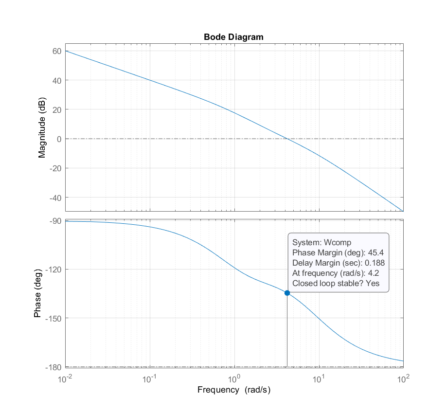
We can see that the phase margin improved. However, it is still 5 degrees less than the desired value of 50 degrees. Consequently, we need to repeat the steps 2,3,4, and 5, by increasing the value of .

This graph is generated by the following MATLAB code:

Gc=tf([a*T 1],[T 1])
Wcomp=Gc*W

figure(3)
bode(Wcomp)

REPETITION OF STEPS 2,3,4, and 5:

Here, we increase the value of to 40. We obtained the following parameters:

(11)  

The compensator is given by

(12)  

The compensated system for this value is shown below.

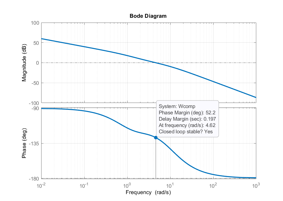
The step response of the compensated system is given below. We can observe that the damping is significantly reduced as well as the settling time.