Control System Tutorial: Definition of Phase Margin and Intuitive Understanding with MATLAB Examples

In this control engineering and control theory tutorial, we introduce the concept of phase margin. We explain how to identify the phase margin from Nyquist and Bode plots. The YouTube video accompanying this post is given below.

Definition of the Phase Margin and Crossover Frequency

Consider an open loop transfer function . Figure 1 below shows the Nyquist plot of the , where and is the frequency. The point is a critical stability point.

Definition of the crossover frequency: The crossover frequency is the frequency at which the Nyquist plot intersects the circle with radius . That is, the crossover frequency is the frequency at which (gain is equal to ), where is the open-loop transfer function in the frequency domain .

Definition of the phase margin: Phase margin is the angle measured in degrees by which the phase of exceeds -180 degrees at . Equivalently, phase margin is an angle in degrees for which the Nyquist plot of needs to be rotated such that the point passes through the point (-1,0).

From mathematical point of view, we have the following relation for the phase margin, that is usually denoted by “PM”:

(1)  

where is the phase of at the crossover frequency .

Intuitive understanding of the phase margin, crossover frequency, and recommendations

Roughly speaking, smaller the phase margin is, more unstable the closed-loop system is. This is because the phase margin is the angle distance from the critical stability point (-1,0). Control engineers ususally specify the desired closed-loop system stability and performance in the form of the phase margin specification. Usually, the lowest acceptable value of the phase margin is PM=30 degrees.

Also, as we will show in the follow-up tutorial, the phase margin is directly related to the damping ratio of the closed-loop system. Higher the phase margin, higher the damping ratio of the closed-loop system. In some sense, the phase margin can be seen as a measure of the robustness of the system. Namely, often in practice, we do not know accurately coefficients of the transfer function. That is, we do not know accurately the system model. By designing systems with sufficiently large phase margins for assumed transfer function parameters, we would ensure that the system remains stable if the actual parameters are different from the assumed parameters that are used to model the system.

The cross-over frequency is the measure of the speed of response of the system.

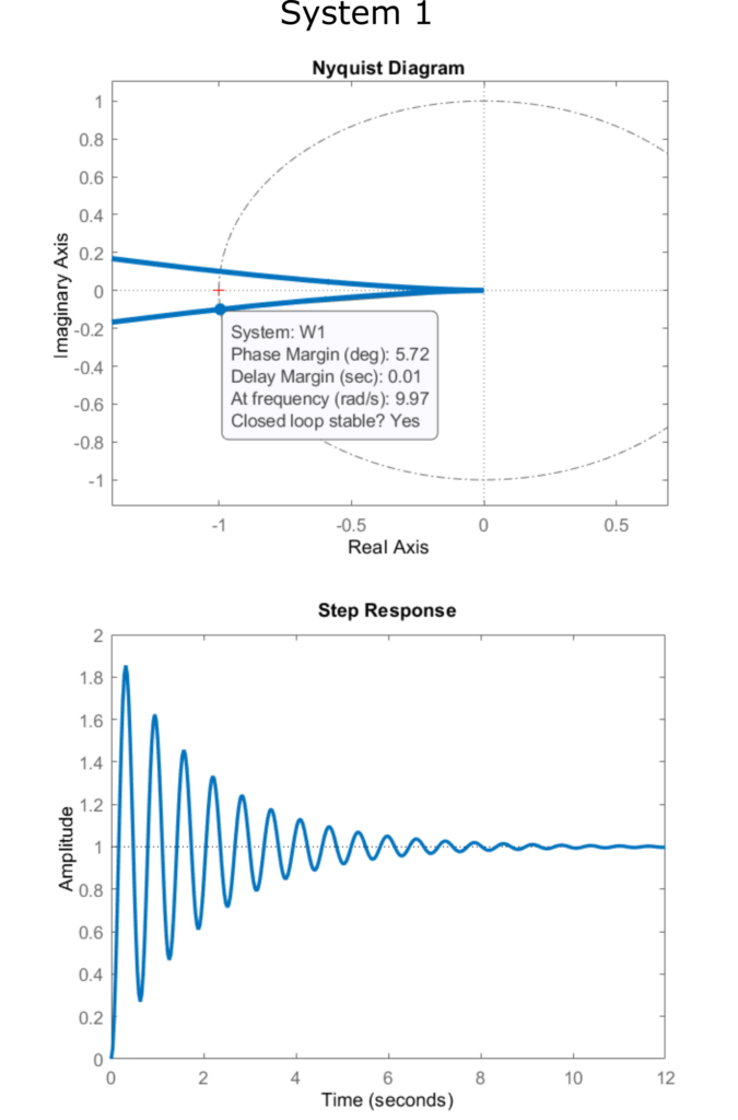
Let us now illustrate graphically how the phase margin influences the transient response and the stability of the system.

We consider three open-loop systems

(2)  

We determine the Nyquist plot and closed-loop step response of these systems by using these MATLAB code lines

W1=tf(1,1*[1 1 0])
nyquist(W1)
W2=feedback(W1,1)

step(W2)

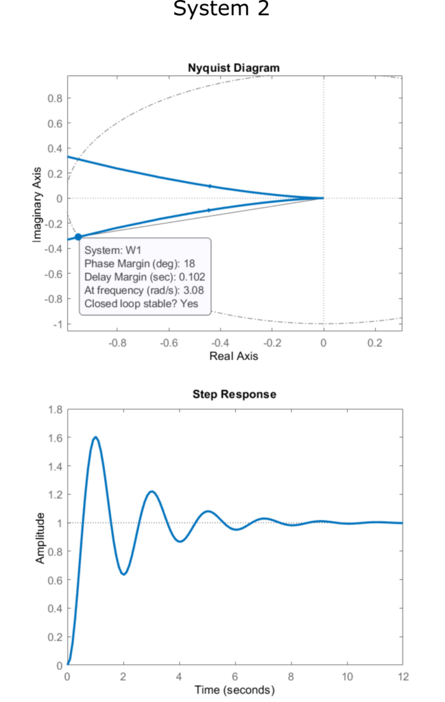
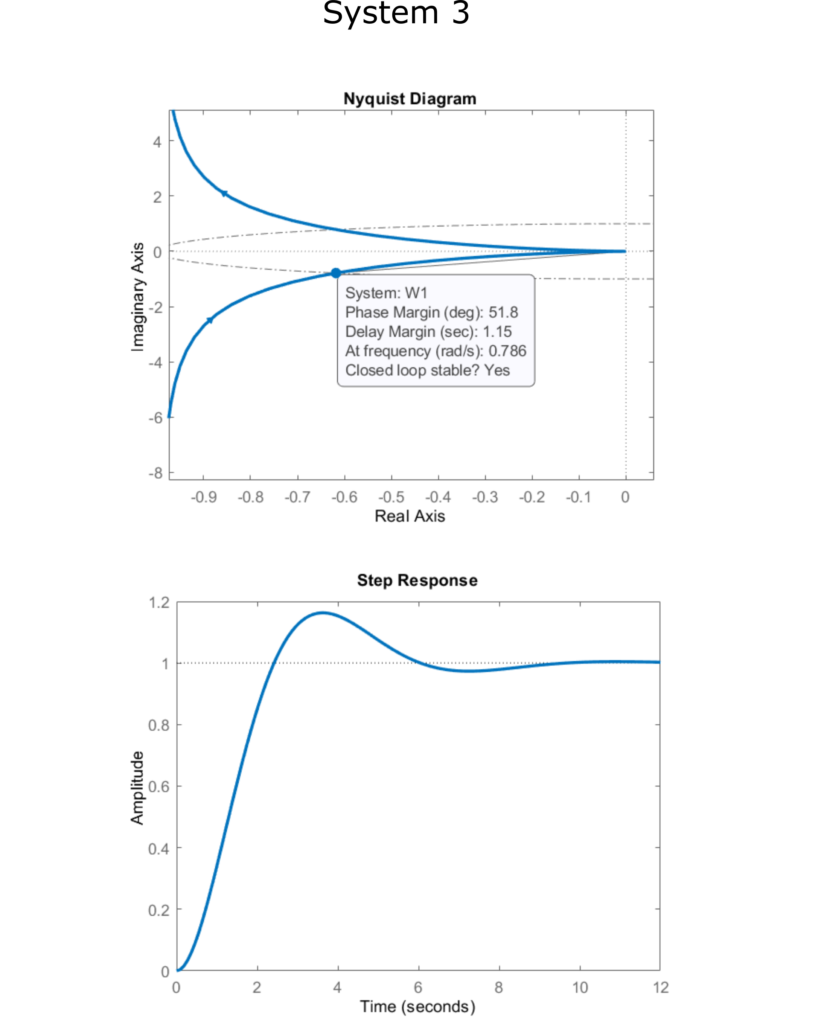
The Nyquist plots of open-loop transfer functions with phase margins together with the corresponding closed-loop step responses of these three systems are shown in the figures below.

Phase Margin from Bode Plot

So far, we learned how to identify the phase margin from the Nyquist plot. Let us now learn how to identify the phase margin from the Bode plot. Consider the following example

(3)  

Let us generate the Bode plot. We use the following MATLAB code lines to generate the Bode plot.

w=tf(1,[1 2 0])
bode(w)

The Bode plot is given in the figure below.

Next, we explain how to identify the phase margin from this plot.

The first step is to draw a horizontal line from the 0 dB and to identify an intersection with the magnitude plot. This is because the phase margin is defined for the point at which . Since the Bode magnitude plot is defined by , we can see that on the Bode plot, the point corresponds to the point at which the magnitude plot crosses the 0 dB point. Then, the next step is to draw a vertical line from this intersection until the -180 horizontal line on the phase plot. The intersection between the vertical line and the phase plot, defines an angle measured from the -180 horizontal line. The angle is positive if the phase plot is above -180, and the angle is negative if the phase plot is below -180. This angle defines the phase margin. This procedure is illustrated in Fig. below.

For the particular example, the phase margin is 76.3 degrees.