Backward Euler Discretization of State-Space Models in MATLAB

In this post, we explain how to implement a backward Euler method in MATLAB for the discretization of state-space models. The backward Euler method has much better stability properties compared to the forward Euler method. However, the backward Euler method is more computationally demanding. The YouTube video accompanying this post is given below

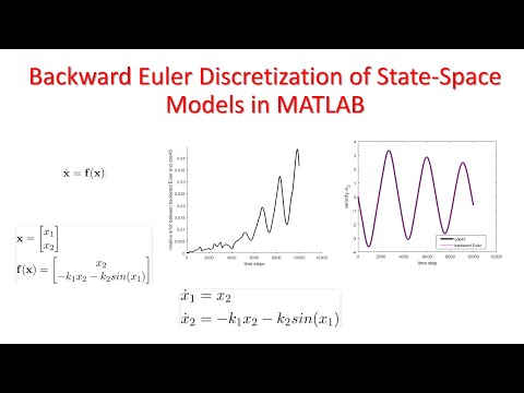
Let us consider a nonlinear pendulum differential equation

(1)  

where is an angle or rotation measured from the vertical axis and and are constants. We introduce state-space variables as follows

(2)  

By using these state-space variables, and by using (1), we can write

(3)  

The last equation can be written compactly

(4)  

where

(5)  

Let denote a discrete-time approximation of the state-space vector , where is a discretization step, and is a discrete-time instant. That is, is a discrete-time approximation of the state-space vector at the time instant .

For a given state-space vector at the time instant , that is, for the given , the backward Euler method computes by solving the following system of nonlinear equations

(6)  

Now, having the initial state , at every iteration , we can obtain the state sequence , by solving the system of nonlinear equations (6). There are several ways for solving the system of equations (6). For example, we can use the Newton, trust-region reflective, or fixed point iteration methods.

Since we are using MATLAB to solve this problem, we write the system of equations (6) in a more appropriate form

(7)  

Let us start with the development of the MATLAB code. First we write a function that describes the system dynamics (3). The function has the following form

% this function defines the dynamics of the system
function dx = dynamics_definition(t,x)
k1=0.1;
k2=5;
dx(1,1)=x(2);
dx(2,1)=-k1*x(2)-k2*sin(x(1));
end

It is important to save this function in a file with the name “dynamics_definition.m”. Also, it is important to add the folder in which this function has been saved to the MATLAB path.

The next step is to define the function that solves the discretized system dynamics by using the backward Euler method. This function has the following form

% - function that simulates the dynamics by using the backward Euler method
%
% - input parameters: 
%                   - time_steps    - discrete-time simulation time 
%                   - x0            - initial state
%                   - h             - discretization constant
%                   - fcnHandle     - function handle that describes the
%                   system dynamics
% - output parameters:
%                   - STATE         - state trajectory
% - Author: Aleksandar Haber
% February 2022

function STATE=solveBackwardEuler(time_steps,x0,h,fcnHandle)
[n,~]=size(x0);
% this is the state trajectory
STATE=zeros(n,time_steps+1);

% here we adjust the options of the MATLAB method for solving nonlinear
% system of equations

% here we set the solver parameters
options_fsolve = optimoptions('fsolve','Algorithm', 'trust-region','Display','off','UseParallel',false,'FunctionTolerance',1.0000e-8,'MaxIter',10000,'StepTolerance', 1.0000e-8);
    
problem.options = options_fsolve;
problem.objective = @objective_fun;
problem.solver = 'fsolve';


for o=1:time_steps
        if o==1
           % the first entry of the STATE trajectory is the initial state
           STATE(:,o)=x0; 
           % generate the initial guess
           problem.x0 = STATE(:,o)+h*fcnHandle(0,STATE(:,o));  % use the Forward Euler method to generate the initial guess
           STATE(:,o+1)=fsolve(problem);
        else
           % generate the initial guess
           problem.x0 = STATE(:,o)+h*fcnHandle(0,STATE(:,o));  % use the Forward Euler method to generate the initial guess
           STATE(:,o+1)=fsolve(problem);
        end
        o
end


% this function defines the backward Euler nonlinear system of equations
% that need to be solved
function f=objective_fun(z)
    f=z-STATE(:,o)-h*fcnHandle(0,z);
end

end

This function has as its inputs the number of discretization steps (“time_steps”), initial state (), discretization constant (h), and a special parameter called “fcnHandle”. The parameter “fcnHandle” is used to denote the name of the function that defined the system dynamics. In our case, the name of the function is “dynamics_definition”. If you have defined the dynamics in a different MATLAB function, then you should use the name of that function.

On code line 23, we specify the optimization parameters. The MATLAB function that will be used to solve the system of nonlinear equations is “fsolve”, and the algorithm is “trust-region”. Then, we define other parameters, such as function tolerances, the maximum number of iterations, step tolerances, and display parameters. Since the problem is low-dimensional we do not use the parallel solver. In fact, in our case, the parallel solver will be much slower than the regular solver. Code lines 25 to 27 are used to finalize the problem definition. Code line 26 specifies the name of the function that defines (7). The actual function is defined in code lines 48-50. Then, the code lines 30 to 43 are defining a for loop that iteratively computes the state trajectories for the discrete-time instants .

The matrix “STATE” stores the state trajectories. The first column is the initial state (code line 33). In the initial iteration , code line 35 is used to define the initial guess of the state vector . We use a forward Euler method to generate that initial guess. The computed value is stored in “problem.x0”. Here it should be emphasized that “problem.x0” is not used to denote the initial state . Instead, this variable is used to store the initial guess for solving the system of equations (7). Code line 36 is actually used to solve the system of nonlinear equations, that are defined by code lines 48-50. In the subsequent iterations 39-40, which are executed for , the initial guess of the solution is updated by using the forward Euler method (code line 39), and the state vector is computed in the code line 40. These iterations are repeated until the maximal number of time steps is reached (variable “time_steps”).

A few additional comments are in order. It is important to emphasize that the function “objective_fun” defined in the code lines 48-50, is able to access the variable “STATE(:,o)” from its parent function. This is a very important fact for the ease of implementation since we do not need to provide this variable as an input to the function.

The function “solveBackwardEuler(time_steps,x0,h,fcnHandle)” is called from the main function defined below:

% simulation of the system dynamics by using the backward Euler
% discretization method
clear, pack, clc

% initial state x0
x0=[2; 0];

% discretization step
h=0.001;

% discrete-time for simulation
simulationTime=0:h:1000*h;

% first simulate the dynamics by using ode45
% we need this simulation in order to evaluate the accuracy of the backward
% Euler method

[ts,stateTrajectoryOde45] = ode45(@dynamics_definition,simulationTime,x0);


% simulate the dynamics by using the backward Euler method
stateTrajectoryBackwardEuler=solveBackwardEuler(length(simulationTime),x0,h,@dynamics_definition);
stateTrajectoryBackwardEuler=stateTrajectoryBackwardEuler';

for i=1:length(simulationTime)
   error_simulation(i)= norm(stateTrajectoryBackwardEuler(i,:)-stateTrajectoryOde45(i,:),2)/norm(stateTrajectoryOde45(i,:),2);
end

figure(1)
hold on
plot(error_simulation,'k');
figure(2)
plot(stateTrajectoryOde45(:,2),'k')
hold on 
plot(stateTrajectoryBackwardEuler(:,2),'m')

First, we define the initial state, discretization step, and simulation time. Then, we simulate the system trajectory by calling the MATLAB function ode45(). This is important since we want to compare our approach with the classical MATLAB approach for solving differential equations. An interested reader might ask us the following questions. Why do we implement our own discretization method when MATLAB already has a built-in function ode45()? Well, the answer is that it is often necessary to build control algorithms where we have explicit control over the method used to discretize the dynamics. Also, the approach presented in this post is a significantly simplified version of the more complex approach that can be used, for example, to develop a control algorithm. Some of the control algorithms are developed by assuming system dynamics in the backward Euler form. Consequently, it is instructive to teach students or interested readers how to implement a simple backward Euler approach in MATLAB.

On code line 22, we call the function “solveBackwardEuler” to discretize the system dynamics by using the backward Euler approach. Then, code lines 25-27 are used to compute the error between the state trajectory obtained by using the MATLAB ode45() function and the state trajectory computed by using the function “solveBackwardEuler”. Then, code lines 29 to 35 are used to plot the error and the two-state trajectories.

The results are given in the figures below.

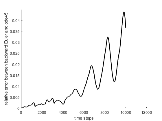
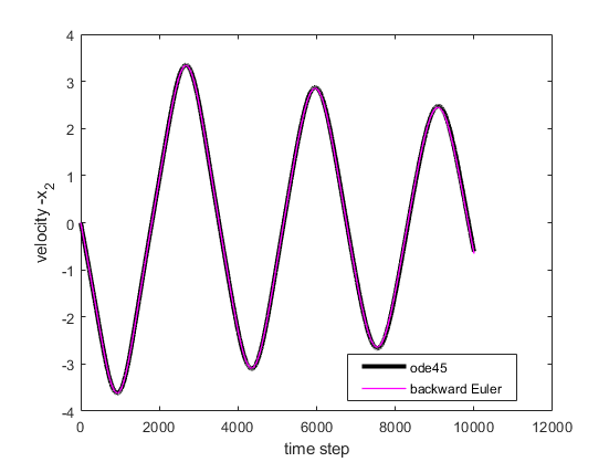
From Fig. 2, we can see that the trajectories are very close to each other. However, from Fig. 1 we can observe that the error increases over time. Several reasons can be behind this. It is possible that the tolerances for obtaining the solution by using ode45 are different from the tolerances used to compute the solution by using the backward Euler method. Another possibility is that the backward Euler method becomes less accurate over time (assuming that the ode45 tolerances are high and that the ode45 computes a more accurate trajectory). That is, it is possible that the discretization errors of the backward Euler method increase over time. If that is the case, then we can decrease the discretization step to obtain more accurate results.