Application of Routh Stability Criterion to Select Parameters of Proportional Integral (PI) Controllers

One of the first problems that we need to solve when designing a control system is to determine allowable values of controller parameters such that the closed-loop system is stable. After this problem is solved, then we can tune these parameters to achieve the desired system performance.

In this post and in the accompanying YouTube video, we explain how to use the Routh stability criterion to determine allowable ranges of proportional and integral control parameters that will ensure that the closed-loop system is stable. The parameters of the derivative control action can be selected at a later stage. The Youtube video accompanying this post is given below.

A basic control structure is shown in Fig. 1 below.

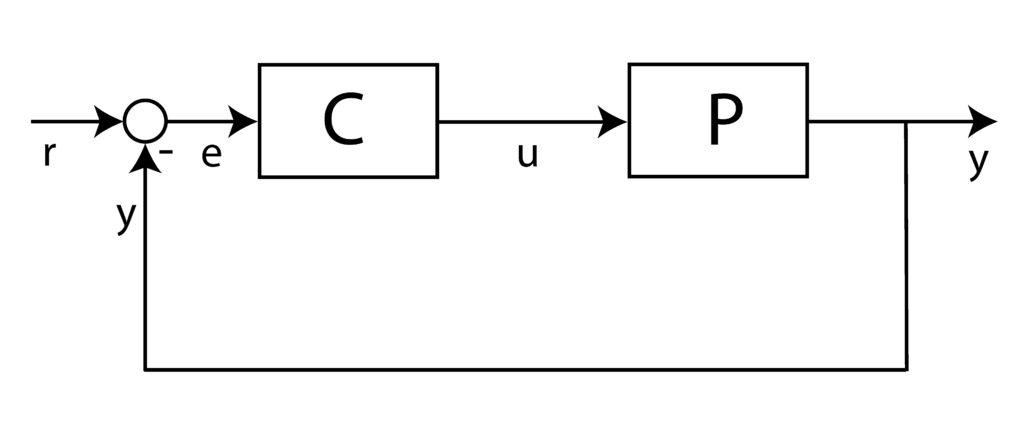
The system that we want to control is denoted by “P” (plant). The controller is denoted by “C”. The reference signal is denoted by and the output of the system is denoted by . The control signal is denoted by . The control error is computed as follows

(1)  

Let us assume that the plant’s model is defined by the following ordinary differential equation of the second order:

(2)  

The Proportional-Integral (PI) control law is given by the following equation

(3)  

where and are proportional and integral control gains. Our goal is to choose the control parameters and such that the closed-loop system is asymptotically stable.

To tackle this problem, we first compute the transfer functions of the plant and controller. The transfer function of the plant is computed from Eq.(2) by performing the Laplace transformation. From Eq.(2) we obtain:

(4)  

where is a complex variable and and are Laplace transforms of and , respectively. We can use the last equation to define a plant transfer function, denoted by , and consequently

(5)  

Similarly, from Eq.(3), we obtain

(6)  

where the and are Laplace transform of and . From Eq.(6), we obtain the controller transfer function

(7)  

The next step is to derive the transfer function of the closed-loop system, denoted by :

(8)  

where is the Laplace transform of . From the block diagram in Fig. 1., we obtain:

(9)  

on the other hand

(10)  

By substituting Eq.(10) in Eq.(9), we obtain

(11)  

and consequently

(12)  

which gives

(13)  

From Eq.(13), we see that the characteristic equation of the closed-loop system is given by

(14)  

By substituting the values for and , that are defined in Eqs. (5) and (6), respectively, in Eq. (14), and by transforming the resulting expression, we obtain

(15)  

The first necessary condition for the system to be asymptotically stable is that all the coefficients of the above polynomial are positive. That is, we need to have

(16)  

Let us now apply the Routh stability criterion in order to determine the ranges of values of and that will render the closed-loop system stable. The Routh array for the third-order characteristic polynomial given in Eq. (15) is

(17)  

According to the Routh stability criterion, the coefficients in the first column have to be positive in order for the closed-loop system to be asymptotically stable.

That is, if

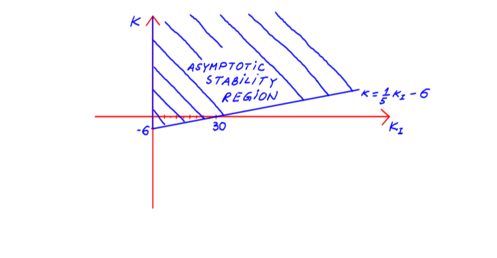
(18)  

then the system is asymptotically stable. The system of inequalities in Eq. (18) define a region in the K_{I}-K plane that is shown in the figure below.

The last step is to verify our theoretical predictions numerically in MATLAB.

The MATLAB code is given below

s = tf('s')

Ki= 1
% this is the boundary: K= (1/5)*Ki-6, stability region is Ki>0 and K> (1/5)*Ki-6 
K= (1/5)*Ki-6+0.21

P=1/(s^2+5*s+6)
C=K+Ki/s

% closed-loop transfer function
W=P*C/(1+P*C)

pole(W)

step(W)

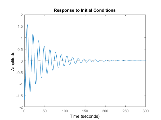
X0=randn(6,1)

initial(ss(W),X0)

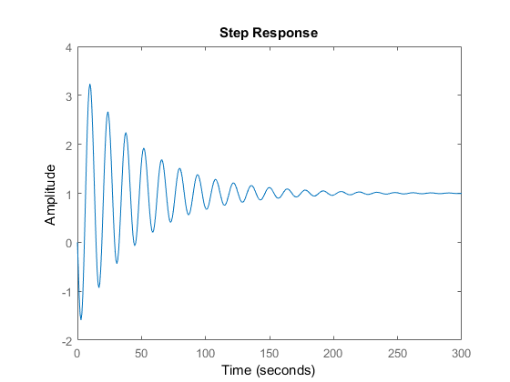
The code lines 1-11 are used to define the closed-loop transfer function. Then, code line 13 is used to compute the closed-loop system poles. The step response of the system is computed and graphed in code line 15. In code line 19, we compute and graph the system response for zero inputs and for the non-zero initial conditions. We have selected the control parameters and such that the system is asymptotically stable. You can easily verify that the system becomes unstable if you select the control parameters to be in the unstable region illustrated in Fig. 1.

The step response is shown in the figure below.

The response of the system to non-zero initial conditions is shown below.